- Research
- Open access
- Published:
Comparison of two projection methods for the solution of frictional contact problems
Boundary Value Problems volume 2019, Article number: 70 (2019)
Abstract
Frictional contact problems in linear elasticity are considered in this paper. The contact constraint is imposed in the weak sense using the fixed point method, which leads to a variational equation problem. For solving such a nonlinear variational problem, we study two projection methods using different self-adaptive rules. Based on the self-adaptive projection method, we propose a modified self-adaptive rule which is more effective to update the parameter. The methods can be implemented easily in conjunction with the boundary element method for the solution. Numerical experiments are reported to illustrate theoretical results.
1 Introduction
Frictional contact phenomena among deformable bodies or between deformable and rigid bodies abound in industry and daily life; they play an important role in many fields of solid mechanics [1, 2]. Because of the nonlinearity, the exact solution is difficult to be obtained. Therefore, a considerable effort has been made in modeling and numerical simulations of contact processes. Most of the time, the mathematical formulation of the frictional contact problem is reformulated as a minimization problem or a variational inequality of the second kind. Theory of contact problems and their numerical approximations has been extensively developed during the past decades [3,4,5,6,7,8,9,10]. Among the most popular methods we mention semi-smooth Newton methods and projection methods. Although the semi-smooth Newton method is well known as the local superlinear convergence for nonlinear problems, this method converges fast only if the penalty parameter of this method is big enough, which may result in a badly conditioned problem; while the projection method with a fixed penalty parameter will be depredated significantly if the parameter is either too small or too large. Therefore, the convergence speed of these methods is sensitive to the choice of parameters. In this paper, we study the numerical solutions of frictional contact problems using the projection method with two self-adaptive rules for the parameter.
The first method, called the self-adaptive projection method in this paper, is applicable for solving monotone variational inequalities of the first kind [9, 11,12,13]. Using the equivalence between the frictional contact problem and a variational formulation with a projection fixed point problem [14,15,16], our method formulates the contact boundary condition into a sequence of Robin boundary conditions. We prove the unconditional convergence in function spaces. The main advantage of the method is that, as compared with other methods, there is a combination of the projection method and the self-adaptive rule which uses iterative functions to update the parameter automatically.
The second method, called the modified self-adaptive projection method in this paper, is based on the self-adaptive projection method. This method uses a modified self-adaptive rule to better adjust the parameter and accelerate the convergence speed of the method, for any initial function. In addition, we note that the proof of the self-adaptive projection method for frictional contact problems can be easily extended to the modified self-adaptive projection method as well.
In these two methods, the key unknowns of frictional contact problems are displacement and stress on the contact boundary, which are considered primary variables and can be related in a linear system by the boundary element method (BEM) [9, 10, 17, 18]. Besides, the BEM significantly reduces expense mesh generation because the formulation of the problem is concluded to the boundary of the domain. Therefore the BEM is a natural numerical tool for the solution of frictional contact problems. In this paper, we apply projection methods combined with the BEM for the numerical solution of frictional contact problems.
The rest of the paper is organized as follows. First, we introduce the variational formulation of the classical frictional contact problem via a projection fixed point problem. Section 3 presents the self-adaptive projection method and the convergence analysis. Section 4 describes the implementation detail of the two self-adaptive rules and the boundary element approximation for the method. In Sect. 5, we give some numerical results that confirm our theoretical findings. In particular, we show that the modified self-adaptive projection method has better convergence speed and stability for all parameters. Finally, Sect. 6 concludes the paper with some remarks.
2 Setting of the problem
We consider the classical frictional contact problem with a rigid foundation. Let Ω be an open and bounded domain in \(\mathbb{R}^{2}\), with a Lipschitz boundary \(\varGamma =\partial \varOmega \). The boundary Γ is partitioned as three mutually disjoint parts \(\varGamma _{D}\), \(\varGamma _{N}\), and \(\varGamma _{C}\neq\varnothing \), where Dirichlet, Neumann, and frictional contact boundary conditions are prescribed. For simplicity, we assume that there are no volume forces acting on the body. We use n and t to denote the outward normal and tangential vectors of Γ, respectively. For given boundary traction \(\hat{\mathbf{t}} \in (L^{2}(\varGamma _{N}))^{2}\) and obstacle \(g \in L^{2}(\varGamma _{C})\) with \(g>0\), the problem is to determine the displacement u such that

and the following friction condition on \(\varGamma _{C}\)

where \(\boldsymbol{u}_{t}\) and \(\boldsymbol{\sigma}_{t}\) are the tangential contact displacement and the tangential contact traction, respectively. In this paper, we adopt the following decomposition for the displacement and the stress vector fields:
Let us introduce the following Hilbert space:
and notations
Problem (2.1)–(2.6) is then equivalent to the following variational inequality of the second kind:
or a convex minimization problem
It follows from the theory of variational inequalities that problem (2.7), or equivalently (2.8), admits a unique solution [1, 2]. Let us introduce a projection notation \([\mathbf{x}]_{\alpha }\) for \(\alpha \in \mathbb{R^{+}}\) and vector \(\mathbf{x}\in \mathbb{R}^{2}\)
Then we have the next result for the frictional boundary condition, which has been pointed out in [15].
Lemma 2.1
For all \(\rho >0\), the frictional contact condition (2.5)–(2.6) on \(\varGamma _{C}\) is equivalent to
Now, we define the following residual function:
As a result, the nonsmooth projection equation (2.9) can be rewritten as \(\boldsymbol{R}_{\rho }(\boldsymbol{u}_{t},\boldsymbol{\sigma}_{t})=\mathbf{0}\). Then, we propose a new equivalent formulation for the frictional boundary condition (2.5)–(2.6). For given \(\omega \ne 0\), \(\boldsymbol{R}_{\rho }( \boldsymbol{u}_{t},\boldsymbol{\sigma}_{t})=\mathbf{0}\) can be written in the following form:
Next, we apply the Green formula to (2.1)–(2.6) and obtain the variational formulation
Consequently, we obtain the following variational and projection formulations for the frictional contact problem (2.1)–(2.6):
Using this equivalent formulation, we can suggest a self-adaptive projection method for the frictional contact problem in the next section.
3 Self-adaptive projection method
In order to solve problem (2.13), we rewrite (2.11) as the following Robin iterative scheme as in [9,10,11,12,13]:
Then we obtain the projection method for the numerical solution of the frictional contact problem. In this method, there are two parameters \(\omega \in (0,2)\) and \(\rho >0\) which affect the convergence speed. We note that the good parameter ω should be less than and close to 2 [9,10,11]. Although the method converges for any fixed parameter \(\rho >0\), the efficiency of the method depends on the parameter ρ heavily.
Here, we propose a projection method with a self-adaptive variable sequence of parameters \(\{\rho _{k}\}\) [9, 10]. In the following we need a nonnegative sequence \(\{s_{k}\}\) satisfying
Now, we present the following self-adaptive projection method for the frictional contact problem.
Algorithm 1
-
Step 0:
Choose initial functions \({\boldsymbol{u}_{t}^{(0)}\in (H^{1/2}(\varGamma _{C}))^{2},\boldsymbol{\sigma}_{t}^{(0)}\in (L^{2}(\varGamma _{C}))^{2}}\), \(\rho \in \mathbb{R^{+}}\), and \(\omega \in (0,2)\); set \(\rho _{0}= \rho \) and \(k:=0\).
-
Step 1:
Compute \(\boldsymbol{R}_{\rho _{k}}(\boldsymbol{u}_{t}^{(k)},\boldsymbol{\sigma}_{t} ^{(k)})\) according to (2.10).
-
Step 2:
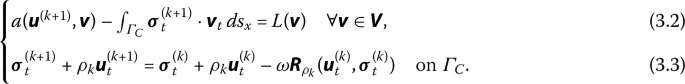
Find \({(\boldsymbol{u}^{(k+1)}, \boldsymbol{\sigma}^{(k+1)})}\) such that
-
Step 3:
Use a self-adaptive rule to update the parameter \(\rho _{k+1}\) satisfying
$$ \frac{1}{1+s_{k}}\rho _{k}\le \rho _{k+1}\le (1+s_{k})\rho _{k}. $$(3.4) -
Step 4:
Stop if some given stopping criterion is satisfied, else set \({k:=k+1}\) and go to Step 1.

Let \(\boldsymbol{u}^{*}\) and \(\boldsymbol{\sigma}^{*}\) denote the solution of the frictional contact problem and the corresponding contact traction on the boundary Γ, respectively. In order to establish the convergence analysis of the projection method, we have to consider preliminary results presented in the form of two lemmas.
Lemma 3.1
If the sequence \(\{s_{k}\}\) satisfies \(s_{k}\ge 0\) and \(\sum\limits_{k=0}^{+\infty }s_{k}<+\infty \), then \(\prod\limits_{k=0}^{+\infty }(1+s _{k})<+\infty \).
Lemma 3.2
Let \((\mathbf{u}^{(k)}, \boldsymbol{\sigma}^{(k)})\) be the sequence generated by the self-adaptive projection method, we have
Lemma 3.1 is obvious and Lemma 3.2 can refer to Theorem 3.3 in [10]. We donate
Consequently, it follows from Step 3 in Algorithm 1 that the parameter \(\rho _{k}\in [\frac{1}{C_{s}}\rho _{0},C_{s}\rho _{0}]\) is bounded. Let
Then, we can prove the following convergence theorem.
Theorem 3.1
Let \(\{(\boldsymbol{u}^{(k)},\boldsymbol{\sigma}^{(k)})\}\) be the sequence generated by the self-adaptive projection method, then \(\mathbf{u}^{(k)}\) converges to \(\mathbf{u}^{*}\) in V and \(\boldsymbol{\sigma}^{(k)}\) converges to \(\boldsymbol{\sigma}^{*}\) in \((L^{2}( \varGamma ))^{2}\).
Proof
Note that \(\boldsymbol{u}^{(k)}\) and \(\boldsymbol{u}^{*}\) satisfy the same boundary conditions on \(\varGamma _{D}\) and \(\varGamma _{N}\). We apply the Green formula to (2.1)–(2.6) and use \(u_{n}^{(k)}=u_{n}^{*}=0\), it follows that
Since \(0<\rho _{k+1}\le (1+s_{k})\rho _{k}\), we use (3.5) and (3.6) and have
Then the following estimation is obtained by using \(\xi _{k}:=2s_{k}+s _{k}^{2}\):
From Lemma 3.1, we have \(\sum_{k=0}^{+\infty }\xi _{k}<+\infty \) and \(\prod_{k=0}^{+\infty }(1+\xi _{k})<+\infty \). We introduce the following notations:
Then \(\boldsymbol{\delta}_{\boldsymbol{u}}^{(k)}\), \(\boldsymbol{\delta}_{\boldsymbol{u}_{t}}^{(k)} \in \boldsymbol{V}\) and \(\boldsymbol{\delta}_{\boldsymbol{\sigma}}^{(k)}\), \(\boldsymbol{\delta} _{\boldsymbol{\sigma}_{t}}^{(k)}\in (L^{2}(\varGamma _{C}))^{2}\). From (3.5) we have
where \(\alpha >0\). Combining (3.7) and (3.8) we get
Therefore, there exists a constant \(\mathrm{C}>0\) such that
Consequently, both sequences \(\{\boldsymbol{u}_{t}^{(k)}\}\) and \(\{ \boldsymbol{\sigma}_{t}^{(k)}\}\) are bounded. From (3.7), we also have
We use (3.8), (3.9), and (3.10) and obtain
Hence, we have
which means that \(\boldsymbol{u}^{(k)}\) converges to \(\boldsymbol{u}^{*}\) in V. From Step 2 of Algorithm 1 and Lebesgue’s bounded convergence theorem it follows that \(\boldsymbol{\sigma}^{(k)}\) converges to \(\boldsymbol{\sigma}^{*}\) in \(L^{2}(\varGamma _{C})\) as \(k\to \infty \). □
4 Implementation details of the proposed method
Consider that our method generates a sequence of well-posed variational problems with the common boundary condition, we can easily obtain their numerical solutions. In this section, we describe the details of the method numerically.
4.1 The self-adaptive rule
Using the method developed in [9,10,11,12,13], we first suggest a simple rule to adjust the variable parameter \(\rho _{k}\) for Step 3 of the self-adaptive projection method. Note that the sequence \(\{(\boldsymbol{u} ^{(k)},\boldsymbol{\sigma}^{(k)})\}\) generated by Algorithm 1 satisfies (3.5) and (3.8), we obtain
For the convergence speed of the method, we hope that
Using this idea, we update the parameter \(\rho _{k}\) as follows. For a given positive constant τ, if
we decrease \(\rho _{k}\) in the next iteration; conversely, we increase \(\rho _{k}\) when
Let
we obtain the parameter \(\rho _{k+1}\) according to the following self-adaptive rule:
where the nonnegative sequence \(\{s_{k}\}\) is generated by
Let \(\mathrm{c}_{k}\) be the change times of \(\{\rho _{k}\}\), i.e.,
For a given constant integer \(\mathrm{c}_{\max}>0\), it follows that the sequence \(\{\mathrm{s}_{k}\}\) satisfies Lemma 3.1 automatically.
4.2 The modified self-adaptive rule
Following the above self-adaptive rule, we use the same way to choose \(\rho _{k+1}\) when \(w_{k}>(1+\tau )\rho _{k}\) and \(w_{k}<\frac{\rho _{k}}{1+ \tau }\). Different from the self-adaptive rule for the case \(\frac{\rho _{k}}{1+\tau }\le w_{k}\le (1+\tau )\rho _{k}\), we give a new rule to adjust \(\rho _{k+1}\) as follows. From (4.1) we have
then we use \(\rho _{k+1}=w_{k}\) to replace \(\rho _{k+1}=\rho _{k}\). Consequently, we obtain the following modified self-adaptive rule:
Obviously, \(\rho _{k+1}\) by using the modified self-adaptive rule also satisfies (3.4). Furthermore, this rule is more flexible to choose a proper parameter and improve the performance of the self-adaptive rule.
4.3 Boundary element discrete form
Problem (3.2)–(3.3) is the variational formulation of the following linear elasticity problem:

Since the main iterative scheme (4.8) is in the boundary of the domain, the BEM is more appropriate for the methods [9, 10, 17, 18].
The solution u of problem (4.4)–(4.8) can be represented as the Betti–Somigliana representation formula
where the x in \(T_{\boldsymbol{x}}\boldsymbol{G}(\boldsymbol{x},\boldsymbol{y})\) denotes differentiations in (4.6) with respect to the variable x, and \(\boldsymbol{G}(\boldsymbol{x},\boldsymbol{y})\) is the fundamental solution of the two-dimensional Lamé equation. The displacements u and tractions Tu satisfy the boundary integral equation
The boundary Γ is approximated by N straight line elements. We use constant boundary elements, and the nodes are located in the middle of each element. Using functions \(\boldsymbol{u}_{t}^{(k)}\) and \(\boldsymbol{\sigma}_{t}^{(k)}\), we obtain the projection residual function \(\boldsymbol{R}_{\rho _{k}}(\boldsymbol{u}_{t}^{(k)},\boldsymbol{\sigma}_{t}^{(k)})\) point-wise on nodes element by element along \(\varGamma _{C}\). We apply \(u_{n}=0\) and the Robin boundary condition
to (4.10) to eliminate \(\sigma _{n}^{(k+1)}\) and obtain the corresponding discrete form at \(\boldsymbol{x}\in \varGamma _{C}\)
On the boundary \(\varGamma _{D}\cup \varGamma _{N}\), the discrete form of the boundary integral equation reads as follows:
Using all the boundary conditions (4.5)–(4.8), we can solve the linear systems (4.12) and (4.13) to obtain both displacement \(\boldsymbol{u}^{(k+1)}\) and stress \(\boldsymbol{\sigma}^{(k+1)}\) at the nodes on Γ. So that we can reset the parameter and the Robin boundary condition on \(\varGamma _{C}\) according to the method.
5 Numerical experiments
In this section, we present some numerical results to compare the performance of the projection method with different self-adaptive rules. In all tests, we take \(\omega =1.8\) and \(\tau =2\), \(c_{\max }=10\) for our methods. Here, we choose \(\frac{\Vert \mathbf{u}^{(k+1)}-\mathbf{u}^{(k)}\Vert _{L^{2}(\varGamma _{C})}+\Vert \boldsymbol{\sigma}_{t}^{(k+1)} -\boldsymbol{\sigma}_{t}^{(k)}\Vert _{L^{2}(\varGamma _{C})}}{ \Vert \mathbf{u}^{(k+1)}\Vert _{L^{2}(\varGamma _{C})}+\Vert \boldsymbol{\sigma}_{t}^{(k+1)} \Vert _{L^{2}(\varGamma _{C})}}\le 10^{-6}\) as a stopping criterion and use Matlab codes for our methods.
5.1 Example 1
We consider an elastic body \(\varOmega =(0,8)\times (0,4)\). The bottom of the rectangle is in contact with a rigid foundation and the frictional contact part of the boundary is \(\varGamma _{C}=(0,8)\times \{0\}\). On the part \(\varGamma _{D}= (0,8)\times \{4\}\) the body is clamped. The Neumann boundary condition is given by \(\hat{\boldsymbol{t}}=(400,0)^{\top }\) on \(\{0\}\times (0,4)\), and \(\hat{\mathbf{t}}={\mathbf{0}}\) on the rest of \(\varGamma _{N}\). The elasticity parameters are chosen to be Young’s modulus \(E=10{,}000\) and Poisson’s ratio \(v=0.3\), the friction coefficient is \(g=150~\mathrm{daN}/\mathrm{mm}^{2}\) on \(\varGamma _{C}\).
First we apply our methods to this problem with initial parameter \(\rho =1\) and step size \(h=0.05\), and the initial and deformed configurations of the body are shown in Fig. 1. On \(\varGamma _{C}\), the tangential displacement and traction are depicted in Figs. 2 and 3, respectively. We note that \(\varGamma _{C}\) is divided into a slip part and a stick part with a transition point from slip to stick near \((3.3, 0)\). It can be seen that our results are in a good agreement with those in Ref. [5].

Initial and deformed configurations

Tangential displacements on \(\varGamma _{C}\)

Tangential tractions on \(\varGamma _{C}\)
Here, we test the problem with different initial positive parameters ρ and mesh sizes h. In Table 1, we give the number of iterations for the convergence of the self-adaptive projection and modified self-adaptive projection methods with rules (4.2) and (4.3), respectively. According to these numerical results, as expected, all parameters ρ do not have a significant effect on the number of iterations for each method. Moreover, the number of iterations for the method depends only weakly on h. In particular, the number of iterations of modified self-adaptive projection method is less than the self-adaptive projection method.
5.2 Example 2
In this example, we consider a frictional problem of the elastic square body \(\varOmega =(0,10)\times (0,2)\) with \(\varGamma _{C}=(0,10)\times \{0\}\). The Neumann boundary condition is given by \(\hat{\boldsymbol{t}}=(1700,0)^{ \top }\) on \(\{0\}\times (0,2)\) and \(\hat{\boldsymbol{t}}=(-1100,0)^{\top }\) on \(\{10\}\times (0,2)\). And the homogeneous Dirichlet condition (i.e., \(\mathbf{u}=\mathbf{0}\)) is applied on \(\varGamma _{D}:=(0,10)\times \{2 \}\). The friction is \(g= 450~\mathrm{daN}/\mathrm{mm}^{2}\) on \(\varGamma _{C}\). Young’s modulus and Poisson’s ratio are \(E=2500\) and \(v=0.2\), respectively.
We choose \(\rho =1\) and \(h=0.05\) again and apply our method to this problem. Figure 4 depicts the initial and deformed configurations of the body, and Figs. 5 and 6 show the surface displacements and stresses on \(\varGamma _{C}\). These numerical results show that \(\varGamma _{C}\) is divided into two slip parts and a stick part with two transition points from slip to stick near \((2.4, 0)\) and \((8.4, 0)\). It can be observed that our results are in agreement with conditions (2.5) and (2.6) again. We also investigate the convergence behavior of our method for this example. Table 2 displays the number of iterations with respect to the parameter ρ and the mesh size h. As in the previous example, our modified self-adaptive projection method is better than the self-adaptive projection method, because this method accelerates the convergence speed.

Initial and deformed configurations

Tangential displacements on \(\varGamma _{C}\)

Tangential tractions on \(\varGamma _{C}\)
6 Conclusion
This paper provides the analysis of two projection methods for the solution of frictional contact problems. Our methods show unconditional convergence and only require solving a sequence of general linear elasticity problems. In particular, we propose two adjustment rules to choose the proper parameter ρ automatically. As the main iterative process is given on the boundary of the domain, the unknowns of the problem are computed easily by using the boundary element method. Furthermore, the numerical results show that the modified self-adaptive projection method has better performance than the self-adaptive projection method. Proposed methods can be extended to frictional contact problems in three space dimensions (3D).
References
Glowinski, R.: Numerical Methods for Nonlinear Variational Problems. Springer, Berlin (2008)
Han, W.M.: A Posteriori Error Analysis Via Duality Theory. Springer, New York (2005)
Stadler, G.: Semismooth Newton and augmented Lagrangian methods for a simplified friction problem. SIAM J. Optim. 15, 39–62 (2004)
De Los Reyes, J.C., Hintermüller, M.: A duality based semismooth Newton framework for solving variational inequalities of the second kind. Interfaces Free Bound. 13, 437–462 (2011)
Bostan, V., Han, W.M.: A posteriori error analysis for finite element solutions of a frictional contact problem. Comput. Methods Appl. Mech. Eng. 195, 1252–1274 (2006)
Denkowski, Z., Migórski, S., Ochal, A.: A class of optimal control problems for piezoelectric frictional contact models. Nonlinear Anal., Real World Appl. 12, 1883–1895 (2011)
Touzaline, A.: Optimal control of a frictional contact problem. Acta Math. Appl. Sin. Engl. Ser. 31, 991–1000 (2015)
Wang, F., Han, W.M., Cheng, X.L.: Discontinuous Galerkin methods for solving a quasistatic contact problem. Numer. Math. 126, 771–800 (2014)
Zhang, S.G., Li, X.L.: A self-adaptive projection method for contact problems with the BEM. Appl. Math. Model. 55, 145–159 (2018)
Zhang, S.G., Li, X.L., Ran, R.S.: Self-adaptive projection and boundary element methods for contact problems with Tresca friction. Commun. Nonlinear Sci. Numer. Simul. 68, 72–85 (2019)
He, B.S., Liao, L.Z., Wang, S.L.: Self-adaptive operator splitting methods for monotone variational inequalities. Numer. Math. 94, 715–737 (2003)
Bnouhachem, A.: An inexact implicit method for general mixed variational inequalities. J. Comput. Appl. Math. 200, 417–426 (2007)
Ge, Z.L., Han, D.R.: Self-adaptive implicit methods for monotone variant variational inequalities. J. Inequal. Appl. 2009, Article ID 458134 (2009)
Chouly, F.: A Nitsche-based method for unilateral contact problems: numerical analysis. SIAM J. Numer. Anal. 51, 1295–1307 (2013)
Chouly, F.: An adaptation of Nitsche’s method to the Tresca friction problem. J. Math. Anal. Appl. 411, 329–339 (2014)
Zhang, S.G., Li, X.L.: An augmented Lagrangian method for the Signorini boundary value problem with BEM. Bound. Value Probl. 2016, 62 (2016)
Hsiao, G.C., Wendland, W.L.: Boundary Integral Equations. Springer, Berlin (2008)
Steinbach, O.: Numerical Approximation Methods for Elliptic Boundary Value Problems. Springer, New York (2008)
Acknowledgements
Not applicable.
Availability of data and materials
All data are fully available without restriction.
Funding
This work is funded by the National Natural Science Foundation Project of CQ CSTC of China (Grant nos. cstc2017jcyjAX0316 and cstc2016jcyjA0419) and the School Fund Project of Chongqing Normal University (CQNU) (Grant no. 16XZH07).
Author information
Authors and Affiliations
Contributions
All authors equally have made contributions. All authors read and approved the final manuscript.
Corresponding author
Ethics declarations
Competing interests
The authors declare that they have no competing interests.
Additional information
Publisher’s Note
Springer Nature remains neutral with regard to jurisdictional claims in published maps and institutional affiliations.
Rights and permissions
Open Access This article is distributed under the terms of the Creative Commons Attribution 4.0 International License (http://creativecommons.org/licenses/by/4.0/), which permits unrestricted use, distribution, and reproduction in any medium, provided you give appropriate credit to the original author(s) and the source, provide a link to the Creative Commons license, and indicate if changes were made.
About this article

Cite this article
Zhang, S., Ran, R. Comparison of two projection methods for the solution of frictional contact problems. Bound Value Probl 2019, 70 (2019). https://doi.org/10.1186/s13661-019-1187-z
Received:
Accepted:
Published:
DOI: https://doi.org/10.1186/s13661-019-1187-z