- Research Article
- Open access
- Published:
Approximate Controllability of a Reaction-Diffusion System with a Cross-Diffusion Matrix and Fractional Derivatives on Bounded Domains
Boundary Value Problems volume 2010, Article number: 281238 (2010)
Abstract
We study the following reaction-diffusion system with a cross-diffusion matrix and fractional derivatives  in
in  ,
,  in
in  ,
,  on
on  ,
,  ,
,  in
in  where
where  is a smooth bounded domain,
  , the diffusion matrix
  has semisimple and positive eigenvalues
  ,
,  ,
,  is an open nonempty set, and
  is the characteristic function of
  . Specifically, we prove that under some conditions over the coefficients
  , the semigroup generated by the linear operator of the system is exponentially stable, and under other conditions we prove that for all
  the system is approximately controllable on
  .
.
1. Introduction
In this paper we prove controllability for the following reaction-diffusion system with cross diffusion matrix:

where  is an open nonempty set of
  and
and  is the characteristic function of
  .
.
We assume the following assumptions.
(H1)  is a smooth bounded domain in
  .
.
(H2) The diffusion matrix  has semisimple and positive eigenvalues
(H3)  are real constants,
  are real constants belonging to the interval
(H4) 
(H5) The distributed controls  .
.
Specifically, we prove the following statements.
(i) If  and
and  , where
  is the first eigenvalue of
  with Dirichlet condition, or if
  , and
, and  then, under the hypotheses (H1)–(H3), the semigroup generated by the linear operator of the system is exponentially stable.
(ii) If  and under the hypotheses (H1)–(H5), then, for all
  and all open nonempty subset
  of
of  the system is approximately controllable on
This paper has been motivated by the work done in [1] and the work done by H. Larez and H. Leiva in [2]. In the work [1], the auther studies the asymptotic behavior of the solution of the system

supplemeted with the initial conditions

The author proved that in the Banach space  where
where  is the space of bounded uniformly continuous real valued functions on
  , if
, if  and
and  are locally Lipshitz and under some conditions over the coefficients
  , and if
  then
then  for all
  Moreover,
  and
and  satisfy the system of ordinary differential equations

with the initial data

The same result holds for 
In the work done in [2], the authers studied the system (1.1) with  , and
, and  They proved that if the diffusion matrix
  has semi-simple and positive eigenvalues
  ,
,  then if
  (
( is the first eigenvalue of
  ), the system is approximately controllable on
  for all open nonempty subset
  of
of 
2. Notations and Preliminaries
In the following we denote by
 the set of
  matrices with entries from
  ,
,
 the set of all measurable functions
  such that
  ,
,
 the set of all the functions
  that have generalized derivatives
  for all
  ,
,
 the closure of the set
  in the Hilbert space
  ,
,
 the set of all the functions
  that have generalized derivatives
  for all
  .
.
We will use the following results.
Theorem 2.1 (cf. [3]).
Let us consider the following classical boundary-eigenvalue problem for the laplacien:

where  is a nonempty bounded open set in
  and
and  .
.
This problem has a countable system of eigenvalues  and
and  as
as  .
.
(i) All the eigenvalues  have finite multiplicity
  equal to the dimension of the corresponding eigenspace
  .
.
(ii) Let  be a basis of the
  for every
  then the eigenvectors
  form a complete orthonormal system in the space
  Hence for all
  we have
  If we put
  then we get
  .
.
(iii) Also, the eigenfunctions  , where
  is the space of infinitely continuously differentiable functions on
  and compactly supported in
  .
.
(iv) For all  we have
  .
.
(v) The operator  generates an analytic semigroup
  on
on  defined by

Definition 2.2.
Let  a real number, the operator
  is defined by

In particular, we obtain  and
and  . Since
  form a complete orthonormal system in the space
  then it is dense in
  , and hence
  is dense in
  .
.
Proposition 2.3 (cf. [4]).
Let  be a Hilbert separable space and
  and
and  two families of bounded linear operators in
  , with
  a family of complete orthogonal projections such that
Define the following family of linear operators  Then
Then
(a)  is a linear and bounded operator if
  with
with  continiuous for
(b) under the above condition (a),  is a strongly continiuous semigroup in the Hilbert space
  whose infinitesimal generator
  is given by

Theorem 2.4 (cf. [5]).
Suppose  is connected,
  is a real function in
  , and
, and  on a nonempty open subset of
  . Then
  in
in  .
.
3. Abstract Formulation of the Problem
In this section we consider the following notations.
-
(i)
 is a Hilbert space with the inner product
 is a Hilbert space with the inner product
 We define

-
(iii)
Let
 then we can define the linear operator
 then we can define the linear operator
where

Therefore, for all 

If we put

then (3.3) can be written as

and we have for all 

Consequently, system (1.1) can be written as an abstract differential equation in the Hilbert space  in the following form:

where  and
and  is a bounded linear operator from
  into
into  .
.
4. Main Results
4.1. Generation of a  -Semigroup
 -Semigroup
Theorem 4.1.
If  , then, under hypotheses (H1)–(H3), the linear operator
  defined by (3.3) is the infinitesimal generator of strongly continuous semigroup
  given by

where


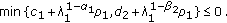
Moreover, if

then the  -semigoup
  is exponentially stable, that is, there exist two positives constants
  such that

Proof.
In order to apply the Proposition 2.3, we observe that  can be written as follows:

where

Therefore,  and
and 
Now, we have to verify condition (a) of the Proposition 2.3. We shall suppose that  Then, there exists a set
  of complementary projections on
  such that

If  is the matrix passage from the canonical basis of
  to the basis composed with the eigenvectors of
  , then

Hence,

We have also

From (4.10)-(4.11) into (4.7) we obtain

where

As  we get

As  as
as  then this implies the existence of a positive number
  and a real number
  such that
  for every
  Therefore
  is a strongly continious semigroup
  given by (4.1). We can even estimate the constants
  and
and  as follows.
-
(i)
If
 As
As  , then there exist constants
 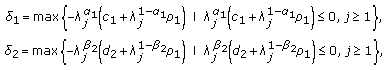 (4.15)
 As
As  , then there exist constants
hence, if we put


we easily obtain

 If
If  . If we put

then we find that

Therefore, the linear operator  generates a strongly continuous semigroup
  on
on  given by expression (4.1).
Finally, if  we have already proved (4.20). Using (4.20) into (4.1) we get that the
  -semigoup
  is exponentially stable. The expression (4.5) is verfied with
  and
and  is defined by (4.19).
Theorem 4.2.
If

then, under the hypotheses (H1)–(H3), the linear operator  defined by (3.3) is the infinitesimal generator of strongly continuous semigroup exponentially stable
  defined by (4.1). Specially, there exist two positives constants
  such that

To prove this result, we need the following lemma.
Lemma 4.3.
For every two real positives constants  and
and  , one has for every

and for every 

Proof of Lemma 4.3.
It is easy to verify that for every  , for all
  .
.
Let  and
and  , then we get

Hence, we get (4.23).
Also, it is easy to verify that for every  , for all
  . Let
. Let  and
and  , then we get

Hence, from  (4.26) we get
  for all
  and
and  , which gives (4.24).
With the same manner we can prove that for every  and every
  we have

and consequently, for every two real positives constants  and
and  and every
  we have

Now, we are ready to prove Theorem 4.2.
Proof of Theorem 4.2.
By applying Proposition 2.3 we start from formula (4.12) and we put

where

To estimate  we have in taking into account

and applying the Lemma 4.3 we get

for all  and
and  . But we have
  , for all
  Then we get for every
  that
that

From (4.31)-(4.33) we get

where

and 
Applying Lemma 4.3 and taking into account (4.21) we get with the same manner that for every 

where

and or every 

where


From (4.34)-(4.40) into (4.12) we get

where  is defined by (4.17) and

Using (4.41) into (4.1) we get that the  -semigoup
  generated by
  is exponentially stable. Expression (4.22) is verfied with
  and
and  is defined by (4.42).
4.2. Approximate Controllability
Befor giving the definition of the approximate controllabiliy for the sytem (3.9), we have the following known result: for all  and
and  the initial value problem (3.9) admits a unique mild solution given by

This solution is denoted by 
Definition 4.4.
System (3.9) is said to be approximately controllable at time  whenever the set
  is densely embedded in
  ; that is,

The following criteria for approximate controllability can be found in [6].
Criteria 1.
System (3.9) is approximately controllable on  if and only if

Now, we are ready to formulate the third main result of this work.
Theorem 4.5.
If the following condition

is satisfied; then, under hypotheses (H1)–(H5), for all  and all open subset
  system (3.9) is approximately controllable on
  .
.
Proof.
The proof of this theorem relies on the Criteria 1 and the following lemma.
Lemma 4.6.
Let and
and  be sequences of real numbers such that
  ,
,  and
and  , for all
  , then for any
  one has

Proof of Lemma 4.6.
By analyticity we get  and from this we get
  . Under the assumptions of the lemma we get
  as
as  and so
  If
If  , we divide
  by
by  and we pass
  we get
  . If
. If  we divide
  by
by  and we pass
  and get
  . If
. If  , we divide
  by
by  and we pass
  and get
  But in this we case we can integrate under the symbol of sommation over the intervall
  and we get
  . Hence
  . Continuing this way we see that
  for all
We are now ready to prove Theorem 4.5. For this purpose, we observe that

where  is the
  -semigroup generated by
  .
.
Without lose of generality, we suppose that  Hence
Hence

where 
Now, suppose for  that
that  , for all
  Then
Then

If (4.46) is satisfied, then (4.50) take the form

Then, from lemma 4.6 we obtain that for  and all

Since  we get that all

On the other hand, from Theorem 2.4 we know that  are analytic functions, which implies the analticity of
  and
and  Then we can conclude that for
  and all

Hence  for all
  which implies that
  This completes the proof of Theorem 4.5.
References
Badraoui S:Asymptotic behavior of solutions to a
 reaction-diffusion system with a cross diffusion matrix on unbounded domains. Electronic Journal of Differential Equations 2006,2006(61):1-13.
Larez H, Leiva H:Interior controllability of a
 a reaction-diffusion system with cross diffusion matrix. to appear in Boundary Value Problems
Zeidler E: Applied Functional Analysis, Applied Mathematical Sciences. Volume 109. Springer, New York, NY, USA; 1995:xvi+404.
Leiva H:A lemma on
 -semigroups and applications. Quaestiones Mathematicae 2003,26(3):247-265. 10.2989/16073600309486057
Axler S, Bourdon P, Ramey W: Harmonic Function Theory, Graduate Texts in Mathematics. Volume 137. Springer, New York, NY, USA; 1992:xii+231.
Curtain RF, Zwart H: An Introduction to Infinite-Dimensional Linear Systems Theory, Texts in Applied Mathematics. Volume 21. Springer, New York, NY, USA; 1995:xviii+698.
 reaction-diffusion system with a cross diffusion matrix on unbounded domains. Electronic Journal of Differential Equations 2006,2006(61):1-13.
 a reaction-diffusion system with cross diffusion matrix. to appear in Boundary Value Problems
 -semigroups and applications. Quaestiones Mathematicae 2003,26(3):247-265. 10.2989/16073600309486057
Author information
Authors and Affiliations
Corresponding author
Rights and permissions
Open Access This article is distributed under the terms of the Creative Commons Attribution 2.0 International License (https://creativecommons.org/licenses/by/2.0), which permits unrestricted use, distribution, and reproduction in any medium, provided the original work is properly cited.
About this article
Cite this article
Badraoui, S. Approximate Controllability of a Reaction-Diffusion System with a Cross-Diffusion Matrix and Fractional Derivatives on Bounded Domains. Bound Value Probl 2010, 281238 (2010). https://doi.org/10.1155/2010/281238
Received:
Accepted:
Published:
DOI: https://doi.org/10.1155/2010/281238