Optimal Conditions for Maximum and Antimaximum Principles of the Periodic Solution Problem

Abstract

Given a periodic, integrable potential , we will study conditions on so that the operator admits the maximum principle or the antimaximum principle with respect to the periodic boundary condition. By exploiting Green functions, eigenvalues, rotation numbers, and their estimates, we will give several optimal conditions.

1. Introduction and Main Results

Maximum Principle (MP) and AntiMaximum Principle (AMP) are fundamental tools in many problems. Generally speaking, criteria for MP and AMP are related to the location of relevant eigenvalues. See, for example, [1–5]. We also refer the reader to Campos et al. [6] for a recent abstract setting of MP and AMP.

In this paper we are studying criteria of MP and AMP for the periodic solution problem of ODEs. For such a problem, MP and AMP are not only related to periodic eigenvalues, but also to antiperiodic eigenvalues. Though there exist several sufficient conditions of MP and AMP for the periodic solution problem in literature like [7–9] (for a brief explanation to these conditions, see Section 4.3), an optimal characterization on MP and AMP is not available. The main aim of this paper is to give several optimal criteria of MP and AMP of the periodic solution problem of ODEs which are expressed using eigenvalues, Green functions, or rotation numbers.

Mathematically, let be the circle of length . Given a -periodic potential , which defines a linear differential operator by

(1.1)

we say that admits the antimaximum principle if

(i) is invertible, and, moreover,

(ii)for any with , one has . Here means that a.e. and on a subset of positive measure.

In an abstract setting, these mean that is a strictly positive operator with respect to the ordering defined by a.e. .

In terminology of differential equations, admits AMP if and only if

(i)for any , the following equation:

(1.2)

has a unique -periodic solution , and, moreover,

(ii)if , one has for all .

We say that admits the maximum principle if for all such that .

Using periodic and antiperiodic eigenvalues of Hill's equations [10, 11], we will obtain the following complete characterizations on MP and AMP.

Theorem 1.1.

Let . Then admits MP iff , and admits AMP iff .

Here and are the smallest -periodic and the smallest -antiperiodic eigenvalues of

(1.3)

respectively. For the precise meaning of these eigenvalues, see Section 2.2.

Given an arbitrary potential , by introducing the parameterized potentials , , Theorem 1.1 can be stated as follows.

Theorem 1.2.

Let . Then admits MP iff , and admits AMP iff .

We will also use Green functions to give complete characterizations on MP and AMP of . See Theorem 4.1 and Corollary 4.4.

The paper is organized as follows. In Section 2, we will briefly introduce some concepts on Hill's equations [10, 12, 13], including the Poincaré matrixes , eigenvalues and rotation numbers and oscillation of solutions. In Section 3, we will use the Poincaré matrixes and fundamental matrix solutions to give the formula of the Green functions of the periodic solution problem (1.2). We will introduce for each potential two matrixes, and , and two functions, and . They are related with the Poincaré matrix and the Green function , respectively. Some remarkable properties on these new objects will be established.

Section 4 is composed of three subsections. At first, in Section 4.1, we will use the sign of Green functions to establish in Theorem 4.1 and Corollary 4.4 optimal conditions for MP and AMP. Then, in Section 4.2, we will use eigenvalues to give a complete description for the sign of Green functions. The proofs of Theorems 1.1 and 1.2 will be given. One may notice that in the deduction of the sign of Green functions, besides eigenvalues, rotation numbers, and oscillation of solutions, some important estimates on Poincaré matrixes in [10, 12] will be used. Moreover, in the deduction of AMP, a very remarkable reduction for elliptic Hill's equations by Ortega [14, 15] is effectively used to simplify the argument. Note that such a reduction is originally used to deduce the formula for the first Birkhoff twist coefficient of periodic solutions of nonlinear, scalar Newtonian equations. Finally, in Section 4.3, we will outline how the known sufficient conditions on AMP can be easily deduced from Theorem 1.1.

2. Basic Facts on Hill's Equations

2.1. Fundamental Solutions and Poincaré Matrixes

Given , let us introduce some basic concepts on the Hill's equation

(2.1)

Let , , be the fundamental solutions of (2.1), that is, are solutions satisfying the initial values

(2.2)

The fundamental matrix solution of (2.1) is

(2.3)

The Liouville theorem asserts that . That is,

(2.4)

the symplectic group of .

The Poincaré matrix of (2.1) is

(2.5)

In particular,

(2.6)

The Floquet multipliers of (2.1) are eigenvalues of . Then , following from (2.6).

We say that (2.1) is elliptic, hyperbolic or parabolic, respectively, if and , , or , respectively. We write the sets of those potentials as , and , respectively.

By introducing the trace

(2.7)

we have the following classification.

Lemma 2.1 (see [10]).

Equaqtion (2.1) is elliptic, hyperbolic, or parabolic, iff , , or , respectively. In particular, implies that .

Proof.

We need to prove the last conclusion. Suppose that . If , we have and . These are impossible.

2.2. Eigenvalues, Rotation Numbers, and Oscillation of Solutions

Given , consider eigenvalue problems of (1.3) with respect to the -periodic boundary condition

(2.8)

or with respect to the -antiperiodic boundary condition

(2.9)

It is well known that one has (real) sequences

(2.10)

such that

(i) and as ;

(ii) is an eigenvalue of problem (1.3)–(2.8) (of problem (1.3)–(2.9), resp.) iff or where is even ( is odd, resp.). Here is void;

(iii) is a periodic (an antiperiodic, resp.) eigenvalue of (1.3) iff

(2.11)

For these general results, one can refer to [10, 11]. Note that in [10] only piecewise continuous potentials are considered. However, these are also true for potentials. See [12, 16].

Denote

(2.12)

Using periodic eigenvalues or traces of Poincaré matrixes, the set can be characterized as

(2.13)

Here the equivalence of (2.13) follows from (2.11).

Let us introduce the rotation number for (2.1). Under the transformation , we know from (2.1) that the argument satisfies

(2.14)

Definition 2.2 (see [17–19]).

Given . Define

(2.15)

where is any solution of (2.14). The limit (2.15) does exist and is independent of the choice of . Such a number is called the rotation number of (2.1). An alternative definition for (2.15) is

(2.16)

where is any nonzero solution of (2.1).

The connection between eigenvalues and oscillation of solutions is as follows.

Lemma 2.3.

Given , consider the parameterized Hill's equations (1.3) where . Then

(i)in case , any nonzero solution of (1.3) is nonoscillatory. More precisely, has at most one zero in the whole line

(ii)in case , any nonzero solution of (1.3) is oscillatory. More precisely, has infinitely many zeros.

2.3. Continuous Dependence on Potentials

Associated with the Hill's equation (2.1), we have the objects , , , and . All are determined by the potential . It is a classical result that all of these objects are continuously dependent on when the topology is considered. For the fundamental matrix solutions, this can be stated as follows.

Lemma 2.4 (see [12, 13]).

Given , the following mapping:

(2.17)

is continuously Frechét differentiable. Moreover, the Frechét derivatives can be expressed using .

In the space , one has also the weak topology which is defined by

(2.18)

In a recent paper [20], Zhang has proved that these objects have stronger dependence on potentials . Some statements of these facts are as follows.

Lemma 2.5 (Zhang [20]).

The following mapping is continuous:

(2.19)

Moreover, the following (nonlinear) functionals:

(2.20)

are also continuous in .

From this lemma, the set is open in and in .

3. Green Functions and Their Variants

3.1. Green Functions

Let . Then, for each , (1.2) has a unique solution satisfying the -periodic boundary condition (2.8). From the Fredholm principle, can be represented as

(3.1)

where

(3.2)

is the so-called Green function of the periodic solution problem (1.2)–(2.8). Another definition of the Green function is

(3.3)

Here is the -periodic unit Dirac measure located at . The Green function can be expressed using and as follows.

Lemma 3.1.

Given , we have the following results.

(i) is given by

(3.4)

(ii) is continuous in and is symmetric

(3.5)

Moreover, can be extended to a continuous -periodic function in both arguments, that is, , .

Proof.

• (i) Formula (3.4) can be found from related references. For completeness, let us give the proof.

Given . By the constant-of-variant formula, solutions of (1.2) are given by

(3.6)

where are constants. In order that is -periodic, it is necessary and sufficient that satisfies (2.8), that is, satisfy

(3.7)

Since , we know that

(3.8)

Hence

(3.9)

where has the form of (3.4).

• (ii) From formula (3.4), the symmetry (3.5) is obvious. Moreover, . Finally, let us show that can be extended to a continuous function on the torus . By using (2.2), (2.5), and (2.6), one has from (3.4)

  

  (3.10)

By the symmetry (3.5), one has

(3.11)

Thus can be understood as a function on .

In general, is not differentiable at the diagonal .

3.2. Two Matrixes and Two Functions

Let us introduce, for any , the following two matrixes:

(3.12)

(3.13)

Note that is a symmetric matrix. Using the Poincaré matrix , and can be rewritten as

(3.14)

Heredenotes the transpose of matrixes, is the identity matrix, and

(3.15)

Some results on and and their connections with the Poincaré matrix are as follows. All of them can be verified directly.

Lemma 3.2.

Given , let , , and . Then

(3.16)

(3.17)

(3.18)

(3.19)

From equalities in Lemma 3.2, we have the following statements.

Lemma 3.3.

Given , then

(i) is nonsingular iff , and is nonsingular iff ;

(ii)Equation (2.1) is elliptic, hyperbolic, or parabolic, iff , , or , respectively.

Since is -periodic, one has the following equality for the fundamental matrix solution

(3.20)

Let us introduce the vector-valued function

(3.21)

which is composed by the fundamental solutions of (2.1). Then

(3.22)

Hence

(3.23)

In the following, we use to denote the Euclidean inner product on . In case , the Green function in (3.4) can be rewritten as

(3.24)

Here is as in (3.12). Note that .

Suggested by (3.24), let us introduce for any two functions

(3.25)

(3.26)

where and are as in (3.12) and (3.13). Note that these functions are well defined on the whole plane and the whole line, respectively. Some properties are as follows.

Lemma 3.4.

For any , one has

(3.27)

(3.28)

(3.29)

Proof.

We need only to verify (3.27) for the case . To this end, one has

(3.30)

For (3.28), we have

(3.31)

Finally, equality (3.29) follows simply from (3.26) and (3.27).

We remark that, in general, is not true for . Note that (3.29) asserts that is -periodic. Some further properties on are as follows.

Lemma 3.5.

• (i) Let . Then does not have any zero and therefore does not change sign.

• (ii) Let . Then has only nondegenerate zeros, if they exist.

• (iii) Let . Then has a constant sign. Moreover,

  

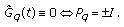  (3.32)

Proof.

• (i) Suppose that is elliptic. We have from Lemma 2.1. By (3.17), . Hence the symmetric matrix is either positive definite or negative definite, according to or . Since for all , we know that on .

• (ii) Suppose that . We have . Thus there exists an orthogonal transformation such that

  

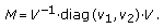  (3.33)

Here are eigenvalues of and satisfy . Then

(3.34)

Note that is also a system of fundamental solutions of (2.1). As , we have

(3.35)

where

(3.36)

Note that is a linearly independent system of solutions of (2.1). From (3.35), has only nondegenerate zeros, if they exist. In fact, suppose that , say . We have and . Thus

(3.37)

• (iii) Suppose that . We have . Then one eigenvalue of is and another is . In this case,

  

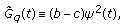  (3.38)

where is a nonzero solution of (2.1). This shows that does not change sign.

We distinguish two cases.

(i) is stable-parabolic, that is, . In this case, one has and .

(ii) is unstable-parabolic, that is, . In this case, we assert that .

Otherwise, assume . Then

(3.39)

Since and , we obtain . Hence and . Moreover, . Thus and is stable-parabolic. In conclusion, for unstable-parabolic case, we have . Now it follows from (3.38) that . As proved before, does not change sign. Moreover, it is easy to see from (3.38) that all zeros of must be degenerate, if they exist.

From these, (3.32) is clear.

4. Optimal Conditions for MP and AMP

4.1. Complete Characterizations of MP and AMP Using Green Functions

Using Green functions , we have the following characterizations on MP and AMP.

Theorem 4.1.

Let with the Green function . Then admits MP iff and

Proof.

We give only the proof for AMP.

The sufficiency is as follows. Suppose that satisfies . Then, for any , it is easy to see from (3.1) that for all . We will show that for all and consequently (1.2) admits AMP.

Otherwise, suppose that for some , that is,

(4.1)

Since , we have necessarily

(4.2)

From (3.24), we know that

(i)on the interval ,

(4.3)

is a solution of (2.1);

(ii)on the interval ,

(4.4)

is also a solution of (2.1).

We assert that these solutions are nonzero when the corresponding intervals are nontrivial. As is composed of two linearly independent solutions , the nontriviality of these solutions is the same as

(4.5)

which are evident because and (3.16) shows that .

From the above assertion, we know that (= has only isolated zeros for . As , we have , a contradiction with (4.2).

For the necessity, let us assume that . Then one has some so that . Hence one has some such that

(4.6)

Let us choose such that

(4.7)

Then . However, the corresponding periodic solution of (1.2) satisfies

(4.8)

Hence does not admit AMP.

In order to apply Theorem 4.1, it is important to compute the signs of the following nonlinear functionals of potentials:

(4.9)

To this end, let us establish some relation between and .

For general , denote

(4.10)

Suppose that so that is meaningful. We assert that

(4.11)

In fact, for , the first case of (4.11) follows immediately from the defining equalities (3.24), (3.25), and (4.10). On the other hand, for , from the second case of (3.24), one has

(4.12)

Hence (4.11) is also true for this case.

By introducing the domain

(4.13)

and the following nonlinear functionals

(4.14)

we have the following statements.

Lemma 4.2.

There hold, for all ,

(4.15)

Proof.

We only prove the first equality of (4.15) because the second one is similar. By (4.11), for any , we have

(4.16)

Hence

(4.17)

Consequently,

(4.18)

This is just (4.15) because .

Remark 4.3.

• (i) The functionals and are well defined for all potentials . Moreover, by (4.15), and have the same signs with the functionals in (4.9).

• (ii) Compared with the defining formulas in (4.9), the novelty of formulas in (4.14) is that when is fixed, is a solution of (2.1), while when is fixed, is also a solution of (2.1). A similar observation is used in [8] as well.

• (iii) Due to the factor which is zero at those , and are in general discontinuous at . However, and are continuous at in the topology or even in the weak topology . See Lemmas 2.4 and 2.5.

By Lemma 4.2, Theorem 4.1 can be restated as follows.

Corollary 4.4.

Let . Then admits MP iff , and admits AMP iff .

4.2. Complete Characterizations of MP and AMP Using Eigenvalues

Lemma 4.5.

Let be such that . Then and admits MP.

Proof.

For simplicity, denote

(4.19)

For any , one has and . See [10]. Thus . In the following let us fix any .

Step 1.

We assert that

(4.20)

Since , we can use the representation (3.35) for where and are nonzero solutions of (2.1). Since , both have at most one zero. See Lemma 2.3. Hence has at most two zeros. However, as is -periodic, does not have any zero. This proves (4.20).

Step 2.

We assert that

(4.21)

If (4.21) is false, there exists such that . By introducing

(4.22)

one has

(4.23)

We know from (3.28) and (4.20) that satisfies

(4.24)

This shows that . Since is a nonzero solution of (2.1), (4.23) implies

(4.25)

Since has the same nonzero value at the end-points of the interval , it is easy to see from (4.24) and (4.25) that must have another zero which is different from . Consequently, the solution of (2.1) has at least zeros and . This is impossible because . See Lemma 2.3.

Step 3.

Let us notice that

(4.26)

We assert that

(4.27)

To prove (4.27), let us fix and consider , where . Then . Since , for all . When , can be estimated. The basic idea is to consider (1.3) as a perturbation of the equation

(4.28)

for which

(4.29)

It is well known that the difference can be controlled by the norm of the potential when . For piecewise continuous and potentials, see [10] and [12], respectively. Similar estimates are also true for potentials. In fact, these can be generalized to Hill's equations with coefficients being measures [16]. We quote from [12, Theorem ] the following result:

(4.30)

Hence

(4.31)

as . We conclude

(4.32)

On the other hand, by (4.21) and (4.26),

(4.33)

Moreover, it follows from Lemma 2.4 that is continuous in . Thus (4.27) follows simply from (4.32) and (4.33).

Step 4.

Since , . It follows from (4.21), (4.26), and (4.27) that, for all , has the same sign with . Thus . By Corollary 4.4, admits MP.

Lemma 4.6.

Suppose that satisfies and . Then and admits AMP.

Proof.

For simplicity, denote

(4.34)

Recall from [11] that eigenvalues and can be characterized using rotation numbers by

(4.35)

Here is arbitrary. Hence

(4.36)

In the following, let . We have , and . Now we argue as in the proof of Lemma 4.5. In this case, result (4.20) can be obtained from Lemma 3.5(i) because . If (4.21) is false at some , we have also . By letting be as in (4.22), one has also some such that and . With loss of generality, let us assume that . Notice that the solution of (2.1) has zeros and . By the Sturm comparison theorem, any nonzero solution of (2.1) has at least one zero in . In particular, for any , is a solution of (2.1). Hence there exists some such that

(4.37)

By equality (3.27),

(4.38)

Thus

(4.39)

From these, the distribution of zeros of the specific solution satisfies

(4.40)

By definition (2.16) for the rotation number, we obtain

(4.41)

a contradiction with the characterization of . Thus (4.21) is also true for .

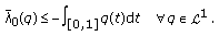
Since , we have from (4.21) and (4.26) that , because we will prove in Lemma 4.7 that for all .

Note that is the set of potentials which are in the first ellipticity zone. By Lemmas 2.1 or 3.5, for all . It seems that there are several ways to deduce that for all . However, some remarkable result on elliptic Hill's equations by Ortega [14, 15] can simplify the argument. Let us describe the result. Suppose that . Consider the temporal-spatial transformation

(4.42)

where and . Then (2.1) is transformed into a new Hill's equation

(4.43)

where is now periodic. The result of Ortega shows that it is always possible to choose some such that the Poincaré matrix (of the period ) of (4.43) is a rigid rotation

(4.44)

See [15, Lemma ] and [21]. We remark that such a result is very important to study the twist character and Lyapunov stability of periodic solutions of nonlinear Newtonian equations and planar Hamiltonian systems. See, for example, [14, 15, 21].

Note that the transformation (4.42) does not change rotation numbers. Recall that the polar coordinates to define rotation numbers are

(4.45)

We see from (4.44) that is related with via

(4.46)

Hence

(4.47)

Lemma 4.7.

We assert that

(4.48)

Proof.

We first prove that , , is invariant under transformations (4.42). In fact, it is well known that and are conjugate

(4.49)

for some . Denote

(4.50)

From (4.49), one has the explicit relation

(4.51)

Note that the quadratic form is definite. See the proof of Lemma 3.5(i). Since , we have

(4.52)

Hence is invariant under transformations (4.42).

Now (4.48) can be obtained as follows. Let . Then . By (4.47), the transformed potential satisfies . By the invariance, we have the desired result (4.48).

Lemma 4.8.

Suppose that satisfies . Then and admits AMP.

Proof.

Since , we have and . See (2.11). Moreover, by (2.10), we have . Let . Then for all . We know from Lemma 4.6 that for . Letting and noticing that is continuous at , we get

(4.53)

On the other hand, let us take an antiperiodic eigen function of (2.1) associated with . Denote by the smallest nonnegative zero of . Then . Moreover, both and are zeros of because of the -antiperiodicity of . By the Sturm comparison theorem, the solution of (2.1) must have some zero in . Hence . As , we obtain

(4.54)

In conclusion we have .

Lemma 4.9.

Suppose that satisfies . Then does not admit neither MP nor AMP.

Proof.

We need not to consider the case because is not invertible.

In the following let us assume that satisfies . Then . The following is a modification of the last part of the proof of Lemma 4.8.

Let us take an antiperiodic eigenfunction associated with . Then the set of all zeros of is for some . Denote

(4.55)

Then is a nonzero solution of (2.1). Since , by applying the Sturm comparison theorem to and , we know that must have some zero in , the interior of the interval because and are consecutive zeros of . As , one must have

(4.56)

Thus changes sign near . Consequently,

(4.57)

Now Corollary 4.4 shows that does not admit AMP. We have also

(4.58)

Hence does not admit MP.

Due to the ordering (2.10) of eigenvalues, the statements in Theorems 1.1 and 1.2 are equivalent. Now let us give the proof of Theorem 1.2. Recall that and for all . By Lemma 4.5, if , admits MP. By Lemmas 4.6 and 4.8, admits AMP for . By Lemma 4.9, does not admit MP nor AMP for . Using the ordering (2.10) for eigenvalues, we complete the proof of Theorem 1.2.

From Lemmas 4.5, 4.6, 4.8, and 4.9, the sign of Green functions is clear in all cases.

Definition 4.10.

Given , we say that admits strong antimaximum principle (SAMP) if admits AMP and, moreover, there exists such that

(4.59)

Then we have the following complete characterizations for SAMP.

Theorem 4.11.

Let . Then admits SAMP iff iff .

4.3. Explicit Conditions for AMP

Let us recall some known sufficient conditions for AMP.

Lemma 4.12 (Torres and Zhang [9]).

Suppose that satisfies the following two conditions:

(4.60)

(4.61)

Then admits AMP.

In the proof there, the positiveness condition (4.60) is technically used extensively. Some optimal estimates on condition (4.61) can be found in Zhang and Li [22]. For an exponent , let us introduce the following Sobolev constant:

(4.62)

Here . These constants can be explicitly expressed using the Gamma function of Euler. The following lower bound for is established in [22]:

(4.63)

where . Hence one sufficient condition for (4.61) is

(4.64)

Now such an condition (4.64) is quite standard in literature like [8, 23], because in case , (4.64) reads as the classical condition

(4.65)

In order to overcome the technical assumption (4.60) on positiveness of , one observation is as follows.

Lemma 4.13 (Torres [8, Theorem ]).

Let . Suppose that all gaps of consecutive zeros of all nonzero solutions of (2.1) are strictly greater than the period 1. Then the Green function has a constant sign.

By Theorem 4.1 of this paper, one sees that the hypothesis in Lemma 4.13 on solutions of (2.1) can yield MP or AMP. Combining ideas from [8, 9, 22], Cabada and Cid have overcome the positiveness condition (4.60) to obtain the following criteria.

Lemma 4.14 (Cabada and Cid [7, Theorem ]).

Suppose that satisfies the following two conditions:

(4.66)

(4.67)

Then admits AMP.

Very recently, Cabada et al. [24, 25] have generalized criteria (4.66)-(4.67) for to AMP of the periodic solutions of the so-called -Laplacian problem

(4.68)

with the constants being replaced by more general Sobolev constants [26].

We end the paper with some remarks.

• (i) Recall the following trivial upper bound:

  

  (4.69)

See, for example, [26]. Criteria (4.66)-(4.67) can be deduced from Theorem 1.1 with the help of estimates (4.63) and (4.69). In fact, by Theorem 4.11, conditions (4.66) and (4.67) guarantee that admits SAMP. For AMP of , condition (4.67) can be improved as

(4.70)

Theorem 1.1 shows that condition (4.61) is optimal, while the complete generalization of condition (4.60) is .

• (ii) It is also possible to construct many potentials for which admits AMP, while (4.70) is violated. For example, let and be defined by

  

  (4.71)

Then and the Riemann-Lebesgue lemma shows that in , where is arbitrarily fixed. In particular, it follows from Lemma 2.5 that

(4.72)

Since

(4.73)

we conclude that for with , admits AMP. However, when is large and ,

(4.74)

is also large. Hence does not satisfy (4.70).

• (iii) Notice that the lower bound (4.63) has actually shown that, under (4.67) ((4.70), resp.), the gaps of consecutive zeros of all nonzero solutions of (2.1) are (, resp.). However, for those potentials as in Theorem 1.1, zeros of solutions of (2.1) may not be so evenly distributed. This is the difference between the sufficient conditions in this subsection and our optimal conditions given in Theorem 1.1.

References

Barteneva IV, Cabada A, Ignatyev AO: Maximum and anti-maximum principles for the general operator of second order with variable coefficients. Applied Mathematics and Computation 2003,134(1):173-184. 10.1016/S0096-3003(01)00280-6
Grunau H-C, Sweers G: Optimal conditions for anti-maximum principles. Annali della Scuola Normale Superiore di Pisa. Classe di Scienze. Serie IV 2001,30(3-4):499-513.
Mawhin J, Ortega R, Robles-Pérez AM: Maximum principles for bounded solutions of the telegraph equation in space dimensions two and three and applications. Journal of Differential Equations 2005,208(1):42-63. 10.1016/j.jde.2003.11.003
Pinchover Y: Maximum and anti-maximum principles and eigenfunctions estimates via perturbation theory of positive solutions of elliptic equations. Mathematische Annalen 1999,314(3):555-590. 10.1007/s002080050307
Takác P: An abstract form of maximum and anti-maximum principles of Hopf's type. Journal of Mathematical Analysis and Applications 1996,201(2):339-364. 10.1006/jmaa.1996.0259
Campos J, Mawhin J, Ortega R: Maximum principles around an eigenvalue with constant eigenfunctions. Communications in Contemporary Mathematics 2008,10(6):1243-1259. 10.1142/S021919970800323X
Cabada A, Cid JÁ: On the sign of the Green's function associated to Hill's equation with an indefinite potential. Applied Mathematics and Computation 2008,205(1):303-308. 10.1016/j.amc.2008.08.008
Torres PJ: Existence of one-signed periodic solutions of some second-order differential equations via a Krasnoselskii fixed point theorem. Journal of Differential Equations 2003,190(2):643-662. 10.1016/S0022-0396(02)00152-3
Torres PJ, Zhang M: A monotone iterative scheme for a nonlinear second order equation based on a generalized anti-maximum principle. Mathematische Nachrichten 2003, 251: 101-107. 10.1002/mana.200310033
Magnus W, Winkler S: Hill's Equation. Dover, New York, NY, USA; 1979:viii+129.
Zhang M:The rotation number approach to eigenvalues of the one-dimensional
-Laplacian with periodic potentials. Journal of the London Mathematical Society. Second Series 2001,64(1):125-143. 10.1017/S0024610701002277
Pöschel J, Trubowitz E: The Inverse Spectrum Theory. Academic Press, New York, NY, USA; 1987.
Zettl A: Sturm-Liouville Theory, Mathematical Surveys and Monographs. Volume 121. American Mathematical Society, Providence, RI, USA; 2005:xii+328.
Ortega R: The twist coefficient of periodic solutions of a time-dependent Newton's equation. Journal of Dynamics and Differential Equations 1992,4(4):651-665. 10.1007/BF01048263
Ortega R: Periodic solutions of a Newtonian equation: stability by the third approximation. Journal of Differential Equations 1996,128(2):491-518. 10.1006/jdeq.1996.0103
Meng G, Zhang M:Measure differential equations, II, Continuity of eigenvalues in measures with
topology. preprint
Feng H, Zhang M: Optimal estimates on rotation number of almost periodic systems. Zeitschrift für Angewandte Mathematik und Physik 2006,57(2):183-204. 10.1007/s00033-005-0020-y
Johnson R, Moser J: The rotation number for almost periodic potentials. Communications in Mathematical Physics 1982,84(3):403-438. 10.1007/BF01208484
Johnson R, Moser J: Erratum: "The rotation number for almost periodic potentials" [Comm. Math. Phys. vol. 84 (1982), no. 3, 403–438]. Communications in Mathematical Physics 1983,90(2):317-318. 10.1007/BF01205510
Zhang M: Continuity in weak topology: higher order linear systems of ODE. Science in China. Series A 2008,51(6):1036-1058. 10.1007/s11425-008-0011-5
Chu J, Lei J, Zhang M: The stability of the equilibrium of a nonlinear planar system and application to the relativistic oscillator. Journal of Differential Equations 2009,247(2):530-542. 10.1016/j.jde.2008.11.013
Zhang M, Li W:A Lyapunov-type stability criterion using
norms. Proceedings of the American Mathematical Society 2002,130(11):3325-3333. 10.1090/S0002-9939-02-06462-6
Chu J, Nieto JJ: Recent existence results for second-order singular periodic differential equations. Boundary Value Problems 2009, 2009:-20.
Cabada A, Cid JÁ, Tvrdý M:A generalized anti-maximum principle for the periodic one-dimensional
-Laplacian with sign-changing potential. Nonlinear Analysis: Theory, Methods & Applications 2010,72(7-8):3436-3446. 10.1016/j.na.2009.12.028
Cabada A, Lomtatidze A, Tvrdý M: Periodic problem involving quasilinear differential operator and weak singularity. Advanced Nonlinear Studies 2007,7(4):629-649.
Zhang M:Certain classes of potentials for
-Laplacian to be non-degenerate. Mathematische Nachrichten 2005,278(15):1823-1836. 10.1002/mana.200410342
Acknowledgments
The author is supported by the Major State Basic Research Development Program (973 Program) of China (no. 2006CB805903), the Doctoral Fund of Ministry of Education of China (no. 20090002110079), the Program of Introducing Talents of Discipline to Universities (111 Program) of Ministry of Education and State Administration of Foreign Experts Affairs of China (2007), and the National Natural Science Foundation of China (no. 10531010).
Author information
Authors and Affiliations
Corresponding author
Rights and permissions
Open Access This article is distributed under the terms of the Creative Commons Attribution 2.0 International License (https://creativecommons.org/licenses/by/2.0), which permits unrestricted use, distribution, and reproduction in any medium, provided the original work is properly cited.
About this article
Cite this article
Zhang, M. Optimal Conditions for Maximum and Antimaximum Principles of the Periodic Solution Problem. Bound Value Probl 2010, 410986 (2010). https://doi.org/10.1155/2010/410986
Received:
Accepted:
Published:
DOI: https://doi.org/10.1155/2010/410986