Singular limiting solutions for elliptic problem involving exponentially dominated nonlinearity and convection term

Abstract

Given Ω bounded open regular set of ℝ² and x₁, x₂, ..., x _m ∈ Ω, we give a sufficient condition for the problem

to have a positive weak solution in Ω with u = 0 on ∂Ω, which is singular at each x _i as the parameters ρ, λ > 0 tend to 0 and where f(u) is dominated exponential nonlinearities functions.

2000 Mathematics Subject Classification: 35J60; 53C21; 58J05.

1 Introduction and statement of the results

We consider the following problem

(1)

where ∇ is the gradient and Ω is an open smooth bounded subset of ℝ². The function a is assumed to be positive and smooth. In the following, we take a(u) = e^λu and f(u) = e^λu(e^u + e^γu), for λ > 0 and γ ∈(0, 1), then problem (1) take the form

(2)

Using the following transformation

then the function w satisfies the following problem

(3)

with ϱ = (λρ²)^1-λ. So when λ → 0⁺, the exponent tends to infinity while the exponent tends to -∞. For ϱ ≡ 0, problem (3) has been studied by Ren and Wei in [1]. See also [2].

We denote by ε the smallest positive parameter satisfying

(4)

Remark that ρ ~ ε as ε → 0. We will suppose in the following

In particular, if we take , then the condition (A _λ ) is satisfied. Under the assumption (A _λ ), we can treat equation (2) as a perturbation of the following:

for γ ∈ (0, 1).

Our question is: Does there exist v_ε,λa sequence of solutions of (2) which converges to some singular function as the parameters ε and λ tend to 0?

In [3], Baraket et al. gave a positive answer to the above question for the following problem

(5)

with a regular bounded domain Ω of ℝ². They give a sufficient condition for the problem (5) to have a weak solution in Ω which is singular at some points (x _i )_1≤i≤mas ρ and λ a small parameters satisfying (A _λ ), where the presence of the gradient term seems to have significant influence on the existence of such solutions, as well as on their asymptotic behavior.

In case λ = 0 the authors in [4] gave also a positive answer for the following problem

(6)

for γ ∈ (0, 1) as ρ tends to 0. When λ = 0 and γ = 0, problem (2) reduce to

(7)

The study of this problem goes back to 1853 when Liouville derived a representation formula for all solutions of (7) which are defined in ℝ², see [5]. It turns out that, beside the applications in geometry, elliptic equations with exponential nonlinearity also arise in modeling many physical phenomenon, such as thermionic emission, isothermal gas sphere, gas combustion, and gauge theory [6]. When ρ tends to 0, the asymptotic behavior of nontrivial branches of solutions of (7) is well understood thanks to the pioneer work of Suzuki [7] which characterizes the possible limit of nontrivial branches of solutions of (7). His result has been generalized in [8] to (6) with , and finally by Ye in [9] to any exponentially dominated nonlinearity f(u). The existence of nontrivial branches of solutions with single singularity was first proved by Weston [10] and then a general result has been obtained by Baraket and Pacard [11]. These results were also extended, applying to the Chern-Simons vortex theory in mind, by Esposito et al. [12] and Del Pino et al. [13] to handle equations of the form -Δu = ρ²V(x)e^u where V is a nonconstant positive potential. See also [14–16] wherever this rule is applicable. where the Laplacian is replaced by a more general divergence operator and some new phenomena occur. Let us also mention that the construction of nontrivial branches of solutions of semilinear equations with exponential nonlinearities allowed Wente to provide counter examples to a conjecture of Hopf [17] concerning the existence of compact (immersed) constant mean curvature surfaces in Euclidean space. Another related problem is the higher dimension problem with exponential nonlinearity. For example, the 4-dimensional semilinear elliptic problem with bi-Laplacian is treated in [18] and the problem with an additional singular source term given by Dirac masses is treated in [19] in the radial case. The results in [18, 19] are generalized to noncritical points of the reduced function, see [20].

We introduce now the Green's function G(x, x') defined on Ω × Ω, to be solution of

and let H(x, x') = G(x, x') + 4log |x - x'|, its regular part. Let m ∈ ℕ, we set

(8)

which is well defined in (Ω)^m for x _i ≠ x _j for i ≠ j. Our main result is the following

Theorem 1 Given β ∈ (0, 1). Let Ω an open smooth bounded set of ℝ², λ > 0 satisfying the condition (A _λ ), γ ∈ (0, 1) and S = {x₁, ... x _m } ⊂ Ω be a nonempty set. Assume that, the point (x₁, ..., x _m ) is a nondegenerate critical point of the function

then there exist ε₀ > 0, λ₀ > 0 and a family of solutions of (2), such that

One of the purpose of the present paper is to present a rather efficient method: nonlinear Cauchy-data matching method to solve such singularly problems. This method has already been used successfully in geometric context (constant mean curvature surfaces, constant scalar curvature metrics, extremal Kähler metrics, manifolds with special holonomy, ...) and appeared in the study [18] in the context of partial differential equations.

2 Construction of the approximate solution

We first describe the rotationally symmetric approximate solutions of

(9)

in ℝ² which will play a central role in our analysis. Given ε > 0, we define

(10)

which is clearly a solution of

(11)

in ℝ². Let us notice that equations (11) is invariant under dilation in the following sense: If v is a solution of (11) and if τ > 0, then v(τ ·) + 2logτ is also a solution of (11). With this observation in mind, we define for all τ > 0

(12)

2.1 A linearized operator on ℝ²

For all ε, τ, λ > 0, we set

(13)

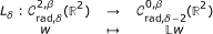
for δ ∈ (0, 1). We define the linear second order elliptic operator

(14)

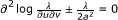
which corresponds to the linearization of (11) about the solution u₁ (= u_{ε = τ = 1}) given by (10) which has been defined in the previous section. We are interested in the classification of bounded solutions of in ℝ². Some solutions are easy to find. For example, we can define

where r = |x|. Clearly and this reflects the fact that (11) is invariant under the group of dilations τ → u(τ ·) + 2 logτ. We also define, for i = 1, 2

which are also solutions of . Since, these solutions correspond to the invariance of the equation under the group of translations a → u(· + a). We recall the following result which classifies all bounded solutions of which are defined in ℝ².

Lemma 1 [11] Any bounded solution of defined in ℝ² is a linear combination of ϕ _i for i = 0, 1, 2.

Let B _r denote the ball of radius r centered at the origin in ℝ².

Definition 1 Given k ∈ ℕ, β ∈ (0, 1) and μ ∈ ℝ, we introduce the Hölder weighted spaces as the space of functions for which the following norm

is finite.

We define also

As a consequence of the result of Lemma 1, we recall the surjectivity result of given in [11].

Proposition 1 [11]

• (i) Assume that μ > 1 and μ ∉ ℕ, then

  

is surjective.

• (ii) Assume that δ > 0 and δ ∉ ℕ then

  

is surjective.

We set , we define

Definition 2 Given k ∈ ℕ, β ∈ (0, 1) and μ ∈ ℝ, we introduce the Hölder weighted spaces as the space of functions in for which the following norm

is finite.

Then, we define the subspace of radial functions in by

We would like to find a solution u of

(15)

in . By using the transformation, then Eq. (15) is equivalent to

(16)

in . We look for a solution of (16) of the form v(x) = u₁(x) + h(x), this amounts to solve

(17)

In . We will need the following:

Definition 3 Given , k∈ ∞, β ∈ (0, 1) and μ ∈ ℝ, the weighted space is defined to be the space of functions endowed with the norm

For all σ ≥ 1, we denote by the extension operator defined by

(18)

where t α χ(t) is a smooth non-negative cutoff function identically equal to 1 for t ≤ 1 and identically equal to 0 for t ≥ 2. It is easy to check that there exists a constant c = c(μ) > 0, independent of σ ≥ 1, such that

(19)

We fix δ ∈ (0, 1) and denote by to be a right inverse of provided by Proposition 1. To find a solution of (17), it is enough to find a fixed point h, in a small ball of , solution of

(20)

We have

This implies that given κ > 0, there exist c _κ > 0 (only depend on κ), such that for δ ∈ (0,1) and |x| = r, we have

Making use of Proposition 1 together with (19), we conclude that

(21)

Now, let h₁, h₂ such that in , then for δ ∈ (0, 1 - r] we have

Similarly, making use of Proposition 1 together with condition (A _λ ) and (19), we conclude that given κ > 0, there exist ε _κ > 0, λ _κ > 0 and (only depend on κ) such that

(22)

Reducing λ _κ > 0 and ε _κ > 0 if necessary, we can assume that, for all λ ∈ (0, λ _κ ) and ε ∈ (0, ε _κ ). Then, (21) and (22) are enough to show that h ↦ ℵ is a contraction from into itself and hence has a unique fixed point h in this set. This fixed point is solution of (20) in . We summarize this in the:

Proposition 2 Given δ ∈ (0, 1 - γ] and κ > 1, then there exist (independent of ε and λ) and a unique with such that

solves (16) in .

2.2 Analysis of the Laplace operator in weighted spaces

In this section, we study the mapping properties of the Laplace operator in weighted Hölder spaces. Given x₁, ..., x _m ∈ Ω, we define x := (x₁, ..., x _m )

and we choose r₀ > 0 so that the balls of center x _i and radius r₀ are mutually disjoint and included in Ω. For all r ∈ (0, r₀), we define

With these notations, we have:

Definition 4 Given k ∈ ℝ, β ∈ (0,1) and ν ∈ ℝ, we introduce the Hölder weighted space as the space of functions for with the following norm

is finite.

When k ≥ 2, we denote by be the subspace of functions satisfying w = 0 on ∂Ω. We recall the

Proposition 3 [21] Assume that ν < 0 and ν ∉ ℤ, then

is surjective. Denote by a right inverse of .

Remark 1 Observe that, when ν < 0, ν ∉ ℤ, the right inverse even though is not unique and can be chosen to depend smoothly on the points x₁, ..., x _m , at least locally. Once a right inverse is fixed for some choice of the points x₁, ..., x _m , a right inverse which depends smoothly on some points close to x₁, ..., x _m can be obtained using a simple perturbation argument. This argument will be used later in the nonlinear exterior problem, since we will move a little bit the points (x _i ).

2.3 Harmonic extensions

We study the properties of interior and exterior harmonic extensions. Given and define Hⁱ (=Hⁱ (φ; ·)) to be the solution of

(23)

We denote by e₁, e₂ the coordinate functions on S¹.

Lemma 2 [21] If we assume that

(24)

then there exists c > 0 such that

Given , we define to be the solution of

(25)

which decays at infinity.

Definition 5 Given k ∈ ℕ, β ∈ (0,1) and ν ∈ ℝ, we define the space as the space of functions for which the following norm

is finite.

Lemma 3 [21] If we assume that

(26)

Then there exists c > 0 such that

If F ⊂ L²(S¹) is a space of functions defined on S¹, we define the space F_⊥ to be the subspace of functions F of which are L²(S¹) -orthogonal to the functions 1, e₁,e₂. We will need the:

Lemma 4 [21] The mapping

where Hⁱ(= Hⁱ (ψ; ·)) and H^e = H^e(ψ; ·), is an isomorphism.

3 The nonlinear interior problem

We are interested in studying equations of type

(27)

In .

Given satisfying (24), we define

Then, we look for a solution of (27) of the form w = v + v and using the fact that Hⁱ is harmonic, this amounts to solve

(28)

We fix μ ∈ (1,2) and denote by to be a right inverse of provided by Proposition 1. To find a solution of (28), it is sufficient to find solution of

(29)

We denote by , the nonlinear operator appearing on the right-hand side of equation (29).

Given κ > 0 (whose value will be fixed later on), we further assume that the functions φ satisfy

(30)

Then, we have the following result

Lemma 5 Given κ > 0. There exist ε _κ > 0, λ _κ > 0, c _κ > 0 and (only depend on κ) such that for all λ ∈ (0, λ _κ ) and ε ∈ (0, ε _κ )

and

provided satisfying .

Proof. The proof of the first estimate follows from the asymptotic behavior of Hⁱ together with the assumption on the norm of boundary data φ given by (30). Indeed, let c _κ be a constant depending only on κ (provided ε and λ are chosen small enough) it follows from the estimate of Hⁱ, given by lemma 2, that

Since for each , we have

where δ ∈ (0, 1 - γ]. Then

On the other hand, using the condition (A _λ ), we have

and

Making use of Proposition 1 together with (20), we get

(31)

In order to derive the second estimate, we use the fact that, for satisfying for i = 1,2, μ ∈ (1,2) and the condition (A _λ ), then there exist c _κ > 0 (only depend on κ) such that

Similarly, making use of Proposition 1 together with (19), we conclude that there exists (only depend on κ) such that

(32)

□

Reducing λ _κ > 0 and ε _κ > 0 if necessary, we can assume that, for all λ ∈ (0, λ _κ ) and ε ∈ (0, ε _κ ). Then, (31) and (32) are enough to show that is a contraction from into itself and hence has a unique fixed point in this set. This fixed point is solution of (20) in ℝ². We summarize this in the following:

Proposition 4 Given κ > 0, there exist ε _κ > 0, λ _κ > 0 and c _κ > 0 (only depending on κ) such that for all ε ∈ (0, ε _κ ), λ ∈ (0, λ _κ ) satisfying (A), for all τ in some fixed compact subset of [τ -, τ⁺] ⊂ (0, ∞) and for a given φ satisfying (24)-(30), then there exists a unique solution of (29) such that

Solve (27) in . In addition,

Observe that the function being obtained as a fixed point for contraction mappings, it depends continuously on the parameter τ.

4 The nonlinear exterior problem

Recall that denote the unique solution of

in Ω, with on ∂Ω. In addition, the following decomposition holds

where is a smooth function. Here, we give an estimate of the gradient of without proof (see [14], Lemma 2.1), there exists a constant c > 0, so that

Let close enough to x := (x₁, ..., x _m ), close to 0 and satisfying (26). We define

(33)

where is a cutoff function identically equal to 1 in and identically equal to 0 outside .

We would like to find a solution of

(34)

in which is a perturbation of . Writing . This amounts to solve

We need to define some auxiliary weighted spaces:

Definition 6 Let , k ∈ ℝ, β ∈ (0, 1) and ν ∈ ℝ, we define the Hölder weighted space as the set of functions for which the following norm

is finite

For all σ ∈ (0, r₀/2) and all Y = (y₁, ..., y _m ) ∈ Ω^m such that ||X - Y || ≤ r₀/2, where X = (x₁, ..., x _m ), we denote by

the extension operator defined by in

for each i = 1, ..., m and in each B_σ/2(y _i ), where is a cutoff function identically equal to 1 for t ≥ 1 and identically equal to 0 for t ≤ 1/2. It is easy to check that there exists a constant c = c(ν) > 0 only depending on ν such that

(35)

We fix

and denote by a right inverse of Δ provided by Proposition 3 with . Clearly, it is enough to find solution of

(36)

where

We denote by the nonlinear operator which appears on the right hand side of Eq.(36). Given κ > 0 (whose value will be fixed later on), we assume that the points , the functions and the parameters to satisfy

(37)

(38)

and

(39)

Then, the following result holds

Lemma 6 Given κ > 0, there exist ε _κ > 0, λ _κ > 0, c _κ > 0 and (depending on κ) such that for all ε ∈ (0, ε _κ ), λ ∈ (0, λ _κ )

and

provided and satisfy .

Proof: Recall that , we will estimate in different subregions of .

* In , we have , and

(40)

so that

Hence, for ν ∈ (- 1, 0) and for small enough, we get

* In , we have and . Thus

So, for ν ∈ (- 1, 0), we have

* In , using the estimat (40), then we have

where

Then

So,

(41)

Making use of Proposition 3 together with (34), we conclude that

(42)

For the proof of the second estimate, let and satisfying for i = 1,2, we have

Then for γ ∈ (0,1), we get

So, for small enough and using the estimate (35), there exist (depending on κ ), such that:

(43)

□

Reducing λ _κ > 0 and ε _κ > 0 if necessary, we can assume that, for all λ ∈ (0, λ _κ ) and ε ∈ (0, ε _κ ). Then, (42) and (43) are enough to show that is a contraction from into itself and hence has a unique fixed point in this set. This fixed point is solution of (35). We summarize this in the following

Proposition 5 Given κ > 0, there exists ε _κ > 0 and λ _κ > 0 (depending on κ) such that for all ε ∈ (0, ε _κ ) and λ ∈ (0, λ _κ ), for all set of parameter satisfying (39) and function satisfying (26), there exists a unique solution of (36) such that

As in the previous section, observe that the function being obtained as a fixed point for contraction mapping, depends smoothly on the parameters and the points .

5 The nonlinear Cauchy-data matching

Keeping the notations of the previous sections, we gather the results of Proposition 4 and 5. Assume that ∈ Ω^m are given close to x := (x₁, ..., x _m ) and satisfy (37). Assume also that τ := (τ₁, ..., τ _m ) ∈ [τ _- , τ ⁺]^m ⊂ (0, ∞)^m are given (the values of τ_- and τ ⁺ will be fixed shortly). First, we consider some set of boundary data satisfying (24). We set

According to the result of Proposition 4, we can find a solution of

(44)

in each that can be decomposed as

where the function satisfies

(45)

Similarly, given some boundary data satisfying (26), some parameters satisfying (38), provide ε ∈ (0, ε _κ ) and λ ∈ (0, λ _κ ), we use the result of Proposition 5, to find a solution v _ext of (43) which can be decomposed as

in where, the function satisfies

(46)

It remains to determine the parameters and the functions in such a way that the function which is equal to in and that is equal to v_ext in is a smooth function. This amounts to find the boundary data and the parameters so that, for each i = 1 ..., m

(47)

on . Assuming we have already done so, this provides for each ε and λ small enough a function (which is obtained by patching together the functions and the function v_ext) solution of -Δv - λ |∇v|² = ρ² (e^v + e^γv) and elliptic regularity theory implies that this solution is in fact smooth. This will complete the proof of our result since, as ε and λ tend to 0, the sequence of solutions we have obtained satisfies the required properties, namely, away from the points x _i the sequence v_ε,λconverges to . Before we proceed, the following remarks are due. First, it will be convenient to observe that the function can be expanded as

(48)

near . The function

which appear in the expression of v _ext can be expanded as

(49)

Near . Here, we have defined

Thus for x near , we have

(50)

where .

Next, in (47), all functions are defined on , but it will be convenient to solve the following equations

(51)

on S¹. Here, all functions are considered as functions of y ∈ S¹ and we have simply used the change of variables to parameterize .

Since the boundary data, we have chosen satisfy (24) and (26), we can decompose

where are constant functions on S¹, belong to and where are L²(S¹) orthogonal to and . Projecting the equations (51) over will yield the system

(52)

Let us comment briefly on how these equations are obtained. They simply come from (51) when expansions (48) and (49) are used, together with the expression of Hⁱ and H^e given in Lemma 2 and Lemma 3, and also the estimates (45) and (46). The system (52) can be readily simplified into

We are now in a position to define τ _- and τ ⁺ since, according to the above, as ε and λ tend to 0 we expect that will converge to x _i and that τ _i will converge to satisfying

and hence, it is enough to choose τ _- and τ ⁺ in such a way that

We now consider the L²-projection of (51) over . Given a smooth function f defined in Ω, we identify its gradient with the element of

With these notations in mind, we obtain the equations

(53)

Finally, we consider the L²-projection onto L²(S¹)^⊥. This yields the system

(54)

Thanks to the result of Lemma 4, this last system can be re-written as

If we define the parameters t = (t _i ) ∈ ℝ^m by

then, the system we have to solve reads

(55)

where as usual, the terms depend nonlinearly on all the variables on the left side, but is bounded (in the appropriate norm) by a constant (independent of ε and λ) time , provide ε ∈ (0, ε _κ ) and λ ∈ (0, λ _κ ). Then, the nonlinear mapping which appears on the right-hand side of (55) is continuous and compact. In addition, reducing ε _κ and λ _κ if necessary, this nonlinear mapping sends the ball of radius (for the natural product norm) into itself, provided κ is fixed large enough. Applying Schauder's fixed Theorem in the ball of radius in the product space where the entries live yields the existence of a solution of Eq. (55) and this completes the proof of our Theorem 1. □

References

Ren X, Wei J: On a two-dimensional elliptic problem with large exponent in nonlinearity. Trans Am Math Soc 1994, 343: 749-763.
Esposito P, Musso M, Pistoia A: Concentrating solutions for a planar problem involving nonlinearities with large exponent. J Diff Eqns 2006, 227: 29-68.
Baraket S, Ben Omrane I, Ouni T: Singular limits solutions for 2-dimensional elliptic problem involving exponential nonlinearities with non linear gradient term. Nonlinear Differ Equ Appl 2011, 18: 59-78.
Baraket S, Ye D: Singular limit solutions for two-dimensional elliptic problems with exponentionally dominated nonlinearity. Chin Ann Math Ser B 2001, 22: 287-296.
Liouville J:Sur l'équation aux différences partielles
. J Math 1853, 18: 17-72.
Tarantello G: Multiple condensate solutions for the Chern-Simons-Higgs theory. J Math Phys 1996, 37: 3769-3796.
Suzuki T: Two dimensional Emden-Fowler Equation with Exponential Nonlinearity. Nonlinear Diffusion Equations and Their Equilibrium States Birkäuser 1992, 3: 493-512.
Nangasaki K, Suzuki T: Asymptotic analysis for two-dimensional elliptic eigenvalue problems with exponentially dominated nonlinearities. Asymptotic Anal 1990, 3: 173-188.
Ye D: Une remarque sur le comportement asymptotique des solutions de - Δ u = λ f ( u ). C R Acad Sci Paris I 1997, 325: 1279-1282.
Weston VH: On the asymptotique solution of a partial differential equation with exponential nonlinearity. SIAM J Math 1978, 9: 1030-1053.
Baraket S, Pacard F: Construction of singular limits for a semilinear elliptic equation in dimension 2. Calc Var Partial Differ Equ 1998, 6: 1-38.
Esposito P, Grossi M, Pistoia A: On the existence of Blowing-up solutions for a mean field equation. Ann I H Poincaré -AN 2005, 22: 227-257.
Del Pino M, Kowalczyk M, Musso M: Singular limits in Liouville-type equations. Calc Var Partial Differ Equ 2005, 24: 47-87.
Wei J, Ye D, Zhou F: Bubbling solutions for an anisotropic Emden-Fowler equation. Calc Var Partial Differ Equ 2007, 28: 217-247.
Wei J, Ye D, Zhou F: Analysis of boundary bubbling solutions for an anisotropic Emden-Fowler equation. Ann I H Poincaré AN 2008, 25: 425-447.
Ye D, Zhou F: A generalized two dimensional Emden-Fowler equation with exponential nonlinearity. Calc Var Partial Differ Equ 2001, 13: 141-158.
Wente HC: Counter example to a conjecture of H. Hopf. Pacific J Math 1986, 121: 193-243.
Baraket S, Dammak M, Ouni T, Pacard F: Singular limits for a 4-dimensional semilinear elliptic problem with exponential nonlinearity. Ann I H Poincaré AN 2007, 24: 875-895.
Dammak M, Ouni T: Singular limits for 4-dimensional semilinear elliptic problem with exponential nonlinearity adding a singular source term given by Dirac masses. Differ Int Equ 2008, 11-12: 1019-1036.
Clapp M, Munoz C, Musso M: Singular limits for the bi-Laplacian operator with exponential nonlinearity in ℝ4. Ann I H Poincaré AN 2008, 25: 1015-1041.
Baraket S, Ben Omrane I, Ouni T, Trabelsi N: Singular limits solutions for 2-dimensional elliptic problem with exponentially dominated nonlinearity and singular data. Communications in Contemporary Mathematics 2 2011, 13(4):129.
Acknowledgements
The authors extend their appreciation to the Deanship of Scientific Research at King Saud University for funding the work through the research group project No RGP-VPP-087.
Author information
Authors and Affiliations
Corresponding author
Additional information
Competing interests
The authors declare that they have no competing interests.
Authors' contribution
The authors declare that the work was realized in collaboration with same responsibility. All authors read and approved the final manuscript.
Rights and permissions
Open Access This article is distributed under the terms of the Creative Commons Attribution 2.0 International License (https://creativecommons.org/licenses/by/2.0), which permits unrestricted use, distribution, and reproduction in any medium, provided the original work is properly cited.
About this article
Cite this article
Baraket, S., Abid, I., Ouni, T. et al. Singular limiting solutions for elliptic problem involving exponentially dominated nonlinearity and convection term. Bound Value Probl 2011, 10 (2011). https://doi.org/10.1186/1687-2770-2011-10
Received:
Accepted:
Published:
DOI: https://doi.org/10.1186/1687-2770-2011-10