Constructive analysis of periodic solutions with interval halving

András Rontó; Miklós Rontó; Nataliya Shchobak

doi:10.1186/1687-2770-2013-57

Research
Open Access
Published: 22 March 2013

Constructive analysis of periodic solutions with interval halving

András Rontó¹,
Miklós Rontó² &
Nataliya Shchobak³

Boundary Value Problems volume 2013, Article number: 57 (2013) Cite this article

2025 Accesses
Metrics details

Abstract

For a constructive analysis of the periodic boundary value problem for systems of non-linear non-autonomous ordinary differential equations, a numerical-analytic approach is developed, which allows one to both study the solvability and construct approximations to the solution. An interval halving technique, by using which one can weaken significantly the conditions required to guarantee the convergence, is introduced. The main assumption on the equation is that the non-linearity is locally Lipschitzian.

An existence theorem based on properties of approximations is proved. A relation to Mawhin’s continuation theorem is indicated.

MSC:34B15.

Introduction

In this paper, we shall develop a numerical-analytic approach to the analysis of periodic solutions of systems of non-autonomous ordinary differential equations using the idea introduced in [1]. The method is numerical-analytic in the sense that its realisation consists of two stages concerning, respectively, an explicit construction of certain equations and their numerical analysis and is close in the spirit to the Lyapunov-Schmidt reductions [2, 3]. However, neither a small parameter nor an implicit function argument is used.

We focus on numerical-analytic schemes based upon successive approximations. In the context of the theory of non-linear oscillations, such types of methods were apparently first developed in [4–8]. We refer the reader to [9–20] for the related bibliography.

For a boundary value problem, the numerical-analytic approach usually replaces the problem by a family of initial value problems for a suitably perturbed system containing a vector parameter which most often has the meaning of the initial value of the solution. The solution of the Cauchy problem for the perturbed system is sought for in an analytic form by successive approximations, whereas the numerical value of the parameter is determined later from the so-called determining equations.

In order to guarantee the convergence, a kind of the Lipschitz condition is usually assumed [9–12] and a smallness restriction of the type

r (K) ≤ q T

(0.1)

is imposed, where K is the Lipschitz matrix and $q T$ depends on the period T. The improvement of condition (0.1) consists in maximising the value of the constant $q T$ .

In this paper, which is a continuation of [1], we provide a constructive approach to the study of solvability of the periodic problem (1.3), (1.4), where the analysis of convergence uses the interval halving technique. We shall see that, under fairly general assumptions, this idea allows one to replace (0.1) by the weaker condition

r (K) ≤ 2 q T

(0.2)

and, thus, significantly improve the convergence conditions established, in particular, in [6–9, 12]. The restriction imposed on the width of the domain is likewise improved. Finally, an existence theorem based upon the properties of approximate solutions is proved. The proofs use a number of technical facts from [1], which are stated in the course of exposition when appropriate.

1 Problem setting and basic assumptions

The method that we are interested in deals with T-periodic solutions of a system of non-linear ordinary differential equations

u ′ (t) = f (t, u (t)), t ∈ (− ∞, ∞),

(1.1)

where $f : R n + 1 → R n$ is a continuous function such that

f (t, z) = f (t + T, z)

(1.2)

for all $z ∈ R n$ and $t ∈ (− ∞, ∞)$ . Here, T is a given positive number. We restrict ourselves to considering continuously differentiable solutions of system (1.1) and, furthermore, instead of T-periodic solutions of (1.1), we shall always deal with the solutions $u : [0, T] → R n$ of the corresponding periodic boundary value problem on the bounded interval $[0, T]$ ,

(1.3)

(1.4)

The passage to problem (1.3), (1.4) is justified by assumption (1.2).

Our main assumption is that $f : [0, T] × R n → R n$ is Lipschitzian with respect to the space variable in a certain bounded set D, which is the closure of a bounded and connected domain in $R n$ . For the sake of simplicity, we assume that there exists a non-negative constant square matrix K of dimension n such that

| f (t, x 1) − f (t, x 2) | ≤ K | x 1 − x 2 |

(1.5)

for all ${x 1, x 2} ⊂ D$ and $t ∈ [0, T]$ .

Here and below, the obvious notation $| x | = col (| x 1 |, | x 2 |, …, | x n |)$ is used, and the inequalities between vectors are understood componentwise. The same convention is adopted implicitly for the operations ‘max’ and ‘min’ so that, e.g., $max {h (z) : z ∈ Q}$ for any $h = (h i) i = 1 n : Q → R n$ , where $Q ⊂ R m$ , $m ≤ n$ , is defined as the column vector with the components $max {h i (z) : z ∈ Q}$ , $i = 1, 2, …, n$ .

2 Notation and symbols

We fix an $n ∈ N$ and a bounded set $D ⊂ R n$ . The following symbols are used in the sequel:

1.
$1 n$ is the unit matrix of dimension n.
2.
$r (K)$ is the maximal, in modulus, eigenvalue of a matrix K.
3.
Given a closed interval $J ⊆ R$ , we define the vector $δ J, D (f)$ by setting
$δ J, D (f) : = max (t, z) ∈ J × D f (t, z) − min (t, z) ∈ J × D f (t, z) .$
(2.1)
4.
$e k$ , $k = 1, 2, …, n$ : see (10.5).
5.
∂ Ω is the boundary of a domain Ω.
6.
$▷ S$ : see Definition 10.1.

The notion of a set $D (r)$ associated with D, which could have been called an inner r-neighbourhood of D, will often be used in what follows.

Definition 2.1 For any non-negative vector $r ∈ R n$ , we put

D (r) : = {z ∈ D : B (z, r) ⊂ D},

(2.2)

where

B (z, r) : = {ξ ∈ R n : | ξ − z | ≤ r} .

(2.3)

One of the assumptions to be used below means that the inner r-neighbourhood of D is non-empty for r sufficiently large.

Finally, let the positive number $ϱ ∗$ be determined by the equality

ϱ ∗ − 1 = inf {q > 0 : q − 1 = ∫ 012 exp (τ (τ − 1) q) d τ} .

(2.4)

We refer, e.g., to [12, 21] for the discussion of other ways of introducing the constant $ϱ ∗$ and for its meaning. What is important for us here is that $ϱ ∗$ is the constant appearing in Lemma 3.2. One can show by computation that

ϱ ∗ ≈ 0.2927 .

(2.5)

3 p-periodic successive approximations

The method suggested by Samoilenko in [6, 7], originally called numerical-analytic method for the investigation of periodic solutions, was also referred to later as the method of periodic successive approximations [9–12]. Its scheme, which is described in a suitable for us form by Propositions 3.1 and 3.4 below, is quite simple and deals with the investigation of the parametrised equation

u (t) = z + ∫ 0 t f (s, u (s)) d s − t T ∫ 0 T f (s, u (s)) d s, t ∈ [0, T],

(3.1)

where $z ∈ D$ is a parameter to be chosen later. For convenience of reference, we formulate the statements for the p-periodic problem

(3.2)

(3.3)

where $g : [t 0, t 0 + p] × R n → R n$ and $t 0 ∈ (− ∞, ∞)$ is arbitrary but fixed.

Following [1], we now describe the original, unmodified, periodic successive approximations scheme for the p-periodic problem (3.2), (3.3) which we are going to modify and which is constructed as follows. With problem (3.2), (3.3), one associates the sequence of functions $u m (⋅, z)$ , $m ≥ 0$ , defined according to the rule

u 0 (t, z) : = z, u m (t, z) : = z + ∫ t 0 t g (s, u m − 1 (s, z)) d s − t − t 0 p ∫ t 0 t 0 + p g (s, u m − 1 (s, z)) d s

(3.4)

for $t ∈ [t 0, t 0 + p]$ and $m = 1, 2, …$ , where the vector $z = col (z 1, z 2, …, z n)$ is regarded as a parameter, the value of which is to be determined later.

Proposition 3.1 ([[12], Theorem 3.17])

Let the function f satisfy the Lipschitz condition (1.5) with a matrix K for which the inequality

r (K) < 1 p ϱ ∗

(3.5)

holds and, moreover,

D (p 4 δ [t 0, t 0 + p], D (g)) ≠ ∅ .

(3.6)

Then, for any fixed $z ∈ D (p 4 δ [t 0, t 0 + p], D (g))$ , the following assertions are true:

1.
Sequence (3.4) converges to a limit function
$u ∞ (t, z) = lim m → ∞ u m (t, z)$
(3.7)

uniformly in $t ∈ [t 0, t 0 + p]$ .

2.
The limit function (3.7) satisfies the p-periodic boundary conditions
$u ∞ (t 0, z) = u ∞ (t 0 + p, z) .$
3.
The function $u ∞ (⋅, z)$ is the unique solution of the Cauchy problem
(3.8)

(3.9)

where

Δ (z) : = ∫ t 0 t 0 + p g (τ, u ∞ (τ, z)) d τ .

(3.10)

4.
Given an arbitrarily small positive ε, one can choose a number $m ε ≥ 1$ such that the estimate
$| u m (t, z) − u ∞ (t, z) | ≤ 12 α m ε (t) K m ε − 1 (ϱ ε p K) m − m ε + 1 (1 n − ϱ ε p K) − 1 δ [t 0, t 0 + p], D (g)$

holds for all $t ∈ [t 0, t 0 + p]$ and $m ≥ m ε$ , where

ϱ ε : = ϱ ∗ + ε .

(3.11)

Recall that, according to (2.2), condition (3.6) means the non-emptiness of the inner $p 4 δ [t 0, t 0 + p], D (g)$ -neighbourhood of the set D, where $δ [t 0, t 0 + p], D (g)$ is the vector given by formula (2.1). This agrees with the natural supposition that, for an approximation technique to be applicable, the domain where the Lipschitz condition is assumed should be wide enough.

The proof of Proposition 3.1 is based on Lemma 3.2 formulated below, which provides an estimate for the sequence of functions $α m$ , $m ≥ 0$ , given by the formula

α m (t) : = (1 − t − t 0 p) ∫ t 0 t α m − 1 (s) d s + t − t 0 p ∫ t t 0 + p α m − 1 (s) d s,

(3.12)

where $m ≥ 1$ and $α 0 (t) : = 1$ , $t ∈ [t 0, t 0 + p]$ . We provide the formulation here for a clearer understanding of the constants appearing in the estimates.

Lemma 3.2 ([[16], Lemma 3])

For any $ε ∈ (0, + ∞)$ , one can specify an integer $m ε ≥ 1$ such that

α m + 1 (t) ≤ p (ϱ ∗ + ε) α m (t)

(3.13)

for all $t ∈ [t 0, t 0 + p]$ and $m ≥ m ε$ .

It should be noted that estimate (3.13) is optimal in the sense that ε can never be put equal to zero.

Remark 3.3 It follows from [[22], Lemma 4] that if $ε ≥ ε 0$ , where

ε 0 : = 310 − ϱ ∗ ≈ 0.00727,

(3.14)

then $m ε = 2$ in Lemma 3.2 (here, of course, we think of $m ε$ as of the least integer possessing the property indicated).

The assertion of Proposition 3.1 suggests a natural way to establish a relation between the p-periodic solutions of the given equation (1.3) and those of the perturbed equation (3.8) (or, equivalently, solutions of the initial value problem (3.8), (3.9)). Indeed, it turns out that, by choosing the value of z appropriately, one can use function (3.7) to construct a solution of the original periodic boundary value problem (1.3), (1.4).

Proposition 3.4 ([1, 12])

Let the assumptions of Proposition 3.1 hold. Then:

1.
Given a $z ∈ D (p 4 δ [t 0, t 0 + p], D (g))$ , the function $u ∞ (⋅, z)$ is a solution of the p-periodic boundary value problem (3.2), (3.3) if and only if z is a root of the equation
$Δ (z) = 0 .$
(3.15)
2.
For any solution $u (⋅)$ of problem (3.2), (3.3) with $u (t 0) ∈ D (p 4 δ [t 0, t 0 + p], D (g))$ , there exists a $z 0$ such that $u (⋅) = u ∞ (⋅, z 0)$ .

The important assertion (2) means that equation (3.15), usually referred to as a determining equation, allows one to track all the solutions of the periodic boundary value problem (1.3), (1.4). In such a manner, the original infinite-dimensional problem is reduced to a system of n numerical equations.

The method thus consists of two parts, namely, the analytic part, when the integral equation (3.1) is dealt with by using the method of successive approximations (3.4), and the numerical one, which consists in finding a value of the unknown parameter from equation (3.15). This closely correlates with the idea of the Lyapunov-Schmidt reduction [2, 3].

The main obstacle for an efficient application of Proposition 3.4 is due to the fact that the function $u ∞ (⋅, z)$ , $z ∈ D (p 4 δ [t 0, t 0 + p], D (g))$ and, therefore, the mapping $Δ : D (p 4 δ [t 0, t 0 + p], D (g)) → R n$ are explicitly unknown. Nevertheless, it is possible to prove the existence of a solution on the basis of the properties of a certain iteration $u m (⋅, z)$ which is constructed explicitly for a certain fixed m. For this purpose, one studies the approximate determining system

Δ m (z) = 0,

(3.16)

where $Δ m : D (p 4 δ [t 0, t 0 + p], D (g)) → R n$ is defined by the formula

Δ m (z) : = ∫ t 0 t 0 + p g (s, u m (s, z)) d s

for $z ∈ D (p 4 δ [t 0, t 0 + p], D (g))$ . This topic is discussed in detail, in particular, in [12], whereas a theorem of the kind specified, which corresponds to the scheme developed here, is proved in Section 9. Our main goal is to obtain a solvability theorem under assumptions weaker than those that would be needed when applying Proposition 3.1.

Indeed, in view of (2.5), assumption (3.5), which is essential for the proof of the uniform convergence of sequence (3.4), can be rewritten in the form

r (K) < p − 1 3.4161 … .

(3.17)

Inequality (3.17) can be treated either as a kind of upper bound for the Lipschitz matrix or as a smallness assumption on the period p, the latter interpretation presenting the scheme as particularly appropriate for the study of high-frequency oscillations.

Without assumption (3.17), Lemma 3.2 does not guarantee the convergence of sequence (3.4) when applied directly along the lines of the proof of Proposition 3.1. Nevertheless, it turns out that this limitation can be overcome and, by using a suitable parametrisation and modifying the scheme appropriately, one can always weaken the smallness condition (3.5) so that the constant on its right-hand side is doubled:

r (K) < 2 p ϱ ∗ .

(3.18)

Note also that, although we have in mind to weaken mainly the smallness condition (3.17) guaranteeing the convergence of iterations, it turns out that the techniques suggested here for this purpose allow us to obtain a considerable improvement of condition (3.6) as well (Corollary 6.7).

Moreover, we shall see that, under the weaker condition (3.18), the modified scheme can be used to prove the existence of a periodic solution on the basis of results of computation (Theorem 10.2).

4 Interval halving, parametrisation and gluing

We should like to show that the approach described by Proposition 3.1 can also be used in the cases where the smallness condition (3.5), which guarantees the convergence, is violated. For this purpose, a natural trick based on the interval halving can be used, where the unmodified scheme, in a sense, should work twice. However, some care should be taken on the boundary conditions.

Indeed, from the first glance, one is tempted to implement halving in the sense that the original scheme should be applied for each of the resulting half-intervals, and thus sequence (3.4) would be constructed twice for problem (3.2), (3.3) with $t 0 = 0$ , $p = 12 T$ , $g = f | [0, 12 T] × R n$ and $t 0 = 12 T$ , $p = 12 T$ , $g = f | [12 T, T] × R n$ , respectively. This is impossible, however, because the boundary conditions on the half-intervals, with trivial exceptions, are never $12 T$ -periodic.

The correct halving scheme is obtained when, along with the periodic boundary value problem (1.3), (1.4), we consider two auxiliary problems

(4.1)

(4.2)

and

(4.3)

(4.4)

where $λ = col (λ 1, …, λ n)$ is a free parameter, the value of which is to be determined suitably from the argument related to gluing. The mutual disposition of the graphs of x and y satisfying, respectively, problems (4.1), (4.2) and (4.3), (4.4) is as shown on Figure 1.

Our further reasoning related to problem (1.3), (1.4) uses the following simple observation. Let us put

χ T (t) : = {1 for 0 ≤ t < 12 T, 0 for 12 T ≤ t ≤ T .

(4.5)

Proposition 4.1 ([1])

Let $x : [0, 12 T] → R n$ and $y : [12 T, T] → R n$ be solutions of problems (4.1), (4.2) and (4.3), (4.4), respectively, with a certain value of $λ ∈ R n$ . Then the function

u (t) : = χ T (t) x (t) + (1 − χ T (t)) (y (t) − y (T 2) + x (T 2)), t ∈ [0, T],

(4.6)

is a solution of the periodic problem boundary value problem (1.4) for the equation

u ′ (t) = f (t, u (t) + (1 − χ T (t)) (y (T 2) − x (T 2))), t ∈ [0, T] .

(4.7)

Conversely, if a certain function $u : [0, T] → R n$ is a solution of problem (1.3), (1.4), then its restrictions $x : = u | [0, 12 T]$ and $y : = u | [12 T, T]$ to the corresponding intervals satisfy, respectively, problems (4.1), (4.2) and (4.3), (4.4).

Remark 4.2 A solution of the functional differential equation (4.7) is understood in the Carathéodory sense, and a jump of $u ′$ at $12 T$ is allowed. Note that function (4.6) is always continuous at $12 T$ .

The idea of Proposition 4.1 is, in fact, to rewrite the periodic boundary condition (1.4) in the form

u (0) − u (T 2) + u (T 2) − u (T) = 0,

(4.8)

which naturally leads us to the introduction of the parameter λ.

Proposition 4.1 allows one to treat the T-periodic problem (1.3), (1.4) as a kind of join of two independent two-point problems (4.1), (4.2) and (4.3), (4.4). Solving them independently and considering λ as an unknown parameter, one can then try to ‘glue’ their solutions together by choosing the value of λ so that (4.9) holds. The possibility of this gluing is equivalent to the solvability of the original problem. A rigorous formulation is contained in the following

Proposition 4.3 ([1])

Assume that $x : [0, 12 T] → R n$ and $y : [12 T, T] → R n$ are solutions of problems (4.1), (4.2) and (4.3), (4.4), respectively, for a certain value of $λ ∈ R n$ . Then the function $u : [0, T] → R n$ given by formula (4.6) is a solution of problem (1.3), (1.4) if and only if the equality

x (T 2) = y (T 2)

(4.9)

holds.

Conversely, if a certain $u : [0, T] → R n$ is a solution of problem (1.3), (1.4), then the functions $x : = u | [0, 12 T]$ and $y : = u | [12 T, T]$ satisfy, respectively, problems (4.1), (4.2) and (4.3), (4.4).

Introduce the functions $α ¯ m : [0, 12 T] → [0, + ∞)$ and $α ¯ ¯ m : [12 T, T] → [0, + ∞)$ , $m ≥ 0$ , by putting $α ¯ 0 ≡ 1$ , $α ¯ ¯ 0 ≡ 1$ ,

α ¯ m + 1 (t) : = (1 − 2 t T) ∫ 0 t α ¯ m (s) d s + 2 t T ∫ t 12 T α ¯ m (s) d s

(4.10)

for $t ∈ [0, 12 T]$ , and

α ¯ ¯ m + 1 (t) : = 2 (1 − t T) ∫ 12 T t α ¯ ¯ m (s) d s + (2 t T − 1) ∫ t T α ¯ ¯ m (s) d s

(4.11)

for $t ∈ [12 T, T]$ . In particular, we have

α ¯ 1 (t) = 2 t (1 − 2 t T), t ∈ [0, 12 T],

(4.12)

and

α ¯ ¯ 1 (t) = 2 (1 − t T) (2 t − T), t ∈ [12 T, T] .

(4.13)

Functions (4.10) and (4.11), which are, in fact, appropriately scaled versions of (3.12), are involved in the estimates given in the sequel.

5 Iterations on half-intervals

As Proposition 4.3 suggests, our approach to the T-periodic problem (1.3), (1.4) requires that we first study the auxiliary problems (4.1), (4.2) and (4.3), (4.4) separately, for which purpose appropriate iteration processes will be introduced. Let us start by considering problem (4.1), (4.2). Following [1], we set

X 0 (t, ξ, λ) : = ξ + 2 t T λ, t ∈ [0, 12 T],

(5.1)

and define the recurrence sequence of functions $X m : [0, 12 T] × R 2 n → R n$ , $m = 0, 1, …$ , by putting

(5.2)

for all $m = 1, 2, …$ , $ξ ∈ R n$ and $λ ∈ R n$ . In a similar manner, for the parametrised problem (4.3), (4.4) on the interval $[12 T, T]$ , we introduce the sequence of functions $Y m : [12 T, T] × R 2 n → R n$ , $m ≥ 0$ , according to the formulae

(5.3)

(5.4)

for all η and λ from $R n$ .

The recurrence sequences determined by equalities (5.1), (5.2) and (5.3), (5.4) arise in a natural way when boundary value problems of type (4.1), (4.1) and (4.3), (4.4) are considered. It is not difficult to verify that formulae (5.1), (5.2) and (5.3), (5.4) are particular cases of those corresponding the iteration scheme for two-point boundary value problems (see, e.g., [23]). One can also derive these formulae directly from Proposition 3.1 by carrying out, respectively, the substitutions $x (t) = u (t) − 2 t T − 1 λ$ , $t ∈ [0, 12 T]$ , and $y (t) = u (t) + (2 t T − 1 − 1) λ$ , $t ∈ [12 T, T]$ , after which one arrives at parametrised $12 T$ -periodic boundary value problems on the corresponding half-intervals.

It is important to note that all the members of the sequences $X m (⋅, ξ, λ)$ , $m ≥ 0$ , and $Y m (⋅, ξ, λ)$ , $m ≥ 0$ , satisfy, respectively, conditions (4.2) and (4.4).

Lemma 5.1 For any ${ξ, η, λ} ⊂ R n$ and $m ≥ 0$ , the functions $X m (⋅, ξ, λ)$ and $Y m (⋅, η, λ)$ satisfy the boundary conditions

(5.5)

(5.6)

Now recall that the vector λ, which is involved in all the above-stated relations, is the ‘gluing’ parameter determining the pair of auxiliary boundary value problems (4.1), (4.2) and (4.3), (4.4), for which a continuous join described by Proposition 4.3 is possible. In this relation, the following property is important.

Lemma 5.2 Let $m ≥ 0$ be arbitrary. Then the equality

X m (T 2, ξ, λ) = Y m (T 2, η, λ)

(5.7)

holds if and only if

λ = η − ξ .

(5.8)

Proof Indeed, it follows directly from (5.1) and (5.3) that $X 0 (12 T, ξ, λ) = ξ + λ$ and $Y 0 (12 T, η, λ) = η$ , whence the assertion is obvious for $m = 0$ . Similarly, if $m ≥ 1$ , then, according to (5.2) and (5.4), we have $X m (12 T, ξ, λ) = ξ + λ$ and $Y m (12 T, η, λ) = η$ and, consequently, relation (5.7) is equivalent to (5.8) for any m. □

6 Successive approximations and their convergence

Let us now pass to the construction of the iteration scheme for the original T-periodic problem (1.3), (1.4). The sequences $X m : [0, 12 T] × R 2 n → R n$ and $Y m : [12 T, T] × R 2 n → R n$ , $m ≥ 0$ , from the preceding section will be used for this purpose. We shall see that, for this purpose, the graphs of the respective members of the last named sequences should be glued together in the sense of Lemma 5.2. Namely, we put

(6.1)

(6.2)

for any $m = 0, 1, …$ . Functions (6.1) and (6.2) will be considered only for those values of ξ and η that are located, in a sense, sufficiently far from the boundary of the domain D. More precisely, we consider $(ξ, η)$ from the set $G D (r)$ , which, for any non-negative vector r, is defined by the equality

G D (r) : = {(ξ, η) ∈ D 2 : B ((1 − θ) ξ + θ η, r) ⊂ D for all θ ∈ [0, 1]} .

(6.3)

Recall that we use notation (2.3). In other words, a couple of vectors $(ξ, η)$ belongs to $G D (r)$ if and only if every convex combination of ξ and η lies in D together with its r-neighbourhood. The inclusion $(ξ, η) ∈ G D (r)$ implies, in particular, that $B (ξ, r) ⊂ D$ and $B (η, r) ⊂ D$ , i.e., the vectors ξ and η both belong to the set $D (r)$ defined by formula (2.2). It is also obvious from (6.3) that $G D (r) ⊂ D 2$ for any r.

The following statement shows that sequence (6.1) is uniformly convergent and its limit is a solution of a certain perturbed problem for all $(ξ, η)$ which are admissible in the sense that $(ξ, η) ∈ G D (r)$ with r sufficiently large.

Theorem 6.1 Let the vector-function $f : [0, T] × D → R n$ satisfy the Lipschitz condition (1.5) on the set D with a matrix K such that

r (K) < 2 T ϱ ∗ .

(6.4)

Moreover, assume that

G D (T 8 δ [0, 12 T], D (f)) ≠ ∅ .

(6.5)

Then, for an arbitrary pair of vectors $(ξ, η) ∈ G D (T 8 δ [0, 12 T], D (f))$ :

1.
The uniform, in $t ∈ [0, 12 T]$ , limit
$lim m → ∞ x m (t, ξ, η) = : x ∞ (t, ξ, η)$
(6.6)

exists and, moreover,

x ∞ (T 2, ξ, η) − x ∞ (0, ξ, η) = η − ξ .

(6.7)

2.
The function $x ∞ (⋅, ξ, η)$ is the unique solution of the Cauchy problem
(6.8)

(6.9)

where

Ξ (ξ, η) : = η − ξ − ∫ 0 T 2 f (τ, x ∞ (τ, ξ, η)) d τ .

(6.10)

3.
Given an arbitrarily small positive ε, one can specify a number $m ε ≥ 1$ such that
(6.11)

for all $t ∈ [0, 12 T]$ and $m ≥ m ε$ , where $ϱ ε$ is given by (3.11).

Recall that the constant $ϱ ∗$ involved in condition (6.4) is given by equality (2.4), while the vector $δ [0, 12 T], D (f)$ arising in (6.5) is defined according to (2.1).

Remark 6.2 The error estimate (6.11) may look inconvenient because it is guaranteed starting from a sufficiently large iteration number, $m ε$ , depending on the value of ε which can be arbitrarily small. It is, however, quite transparent when the required constant is not ‘too close’ to $ϱ ∗$ (i.e., if ε is not ‘too small’). More precisely, in view of Remark 3.3, $m ε = 2$ for $ε ≥ ε 0$ , where

ε 0 ≈ 0.00727

is given by formula (3.14). Consequently, inequality (6.11) with $ε ≥ ε 0$ holds for an arbitrary value of $m ≥ 2$ .

By analogy with Theorem 6.1, under similar conditions, we can establish the uniform convergence of sequence (6.2). Namely, the following statement holds.

Theorem 6.3 Assume that the vector-function f satisfies conditions (1.5), (6.4) and, moreover,

G D (T 8 δ [12 T, T], D (f)) ≠ ∅ .

(6.12)

Then, for all fixed $(ξ, η) ∈ G D (T 8 δ [12 T, T], D (f))$ :

1.
The uniform, in $t ∈ [12 T, T]$ , limit
$lim m → ∞ y m (t, ξ, η) = : y ∞ (t, ξ, η)$
(6.13)

exists and, moreover,

y ∞ (T, ξ, η) − y ∞ (T 2, ξ, η) = ξ − η .

(6.14)

2.
The function $y ∞ (⋅, ξ, η)$ is the unique solution of the Cauchy problem
(6.15)

(6.16)

where

H (ξ, η) : = ξ − η − ∫ T 2 T f (τ, y ∞ (τ, ξ, η)) d τ .

(6.17)

3.
For an arbitrarily small positive ε, one can find a number $m ε ≥ 1$ such that
(6.18)

for all $t ∈ [12 T, T]$ and $m ≥ m ε$ , where $ϱ ε$ is given by (3.11).

Remark 6.4 Similarly to Remark 6.2, one can conclude that the validity of estimate (6.18) is ensured for all $m ≥ 1$ provided that $ε ≥ ε 0$ with $ε 0$ given by formula (3.14).

Theorems 6.1 and 6.3 are improved versions of Theorems 1 and 2 from [1], and their proofs follow the lines of those given therein. The main difference here is the use of Lemma 7.2 in order to guarantee that the values of the iterations do not escape from D. The rest of the argument is pretty similar to that of [1], and we omit it.

Note that the assumptions of Theorems 6.1 and 6.3 differ from each other in conditions (6.5) and (6.12) only. Therefore, by putting

r D (f) : = T 8 max {δ [0, 12 T], D (f), δ [12 T, T], D (f)},

(6.19)

we arrive immediately at the following statement summarising the last two theorems.

Theorem 6.5 Assume that the function f satisfies the Lipschitz condition (1.5) in D with K satisfying relation (6.4) and, moreover, D is such that

G D (r D (f)) ≠ ∅ .

(6.20)

Then, for any $(ξ, η) ∈ G D (r D (f))$ , the assertions of Theorems 6.1 and 6.3 hold.

Recall that D is the main domain where the Lipschitz condition (1.5) is assumed, whereas $G D (r D (f))$ is the subset of $D 2$ defined according to (6.3). The latter set is, in a sense, a two-dimensional analogue of $D (r D (f))$ and, as has already been noted above, the inclusion

G D (r D (f)) ⊂ D (r D (f)) × D (r D (f))

(6.21)

is true. By virtue of (6.21), assumption (6.20) implies in particular that

D (r D (f)) ≠ ∅,

(6.22)

which is a condition of type (3.6) appearing in Proposition 3.1 (see Figure 2). It turns out that, in the case of a convex domain, condition (6.20) can always be replaced by (6.22). Indeed, the following statement holds.

Lemma 6.6 If the domain D is convex, then the corresponding set $G D (r D (f))$ has the form

G D (r D (f)) = D (r D (f)) × D (r D (f)) .

Proof In view of (6.21), it is sufficient to show that

G D (r D (f)) ⊃ D (r D (f)) × D (r D (f)) .

(6.23)

Indeed, let us put $r : = r D (f)$ (the assertion is, of course, true for any non-negative vector r, but the present formulation is sufficient for our purposes) and assume that, on the contrary, inclusion (6.23) does not hold. Then one can specify some ξ and η such that

(6.24)

(6.25)

According to definition (6.3), relation (6.25) means the existence of certain $θ 0 ∈ [0, 1]$ and $z ∈ R n$ such that

z ∈ B ((1 − θ 0) ξ + θ 0 η, r) ∖ D .

(6.26)

Let us put $h : = z − (1 − θ 0) ξ − θ 0 η$ . Then, in view of (6.26), we have

| h | ≤ r .

(6.27)

Furthermore, it is obvious that

(1 − θ 0) (ξ + h) + θ 0 (η + h) = z

(6.28)

and, consequently, z is a convex combination of $ξ + h$ and $η + h$ . By virtue of (2.2), (6.24) and (6.27), both vectors $ξ + h$ and $η + h$ belong to D and, therefore, so does z because (6.28) holds and the set D is convex. However, this contradicts relation (6.26). Thus, inclusion (6.23) holds, and our lemma is proved. □

By virtue of Lemma 6.6, the assertion of Theorem 6.5 for f Lipschitzian in a convex domain can be reformulated as follows.

Corollary 6.7 Let f satisfy conditions (1.5) and (6.4). If, moreover, the domain D is convex and (6.22) holds, then, for any ξ and η from $D (r D (f))$ , all the assertions of Theorems 6.1 and 6.3 hold.

The convexity assumption on D is rather natural and, in fact, the domain where the Lipschitz condition for the non-linearity is verified most frequently has the form of a ball (in our case, where the inequalities between vectors are understood componentwise, it is an n-dimensional rectangular parallelepiped).

We note that the smallness assumption (6.4), which guarantees the convergence of iterations in Corollary 6.7, is twice as weak as the corresponding condition (3.5) of Proposition 3.1:

r (K) < 1 T ϱ ∗ .

(6.29)

Furthermore, it is rather interesting to observe that the condition on inner neighbourhoods also becomes less restrictive after the interval halving has been carried out. Indeed, it is clear from (2.1) and (6.19) that, for condition (6.22) of Corollary 6.7 to be satisfied, it would be sufficient if

D (T 8 δ [0, T], D (f)) ≠ ∅,

(6.30)

whereas, at the same time, assumption (3.6) of Proposition 3.1 would require the relation

D (T 4 δ [0, T], D (f)) ≠ ∅ .

(6.31)

The radius of the inner neighbourhood in (6.30) is less by half. Comparing (6.4) and (6.30) with the corresponding conditions (6.29) and (6.31) arising in Proposition 3.1, we conclude that the idea of interval halving described above thus allows us to improve the original scheme of periodic successive approximations in both directions.

Theorem 6.5 suggests that the iteration sequences (5.2) and (5.4) can be used to construct the solutions of auxiliary problems (4.1), (4.2) and (4.3), (4.4) and ultimately of the original problem (1.3), (1.4). A further analysis, which will lead us to an existence theorem, involves determining equations. Before continuing, we give some auxiliary statements.

7 Auxiliary statements

Several technical lemmata given below are needed in the proof of Theorems 6.1 and 6.3. We implicitly assume in the formulations that condition (6.20) is satisfied.

Given arbitrary $i ∈ {0, 1}$ and $v ∈ C ([12 i T, 12 (i + 1) T], R n)$ , put

(P i v) (t) : = ∫ i 2 T t v (s) d s − (2 t T − i) ∫ i 2 T i + 1 2 T v (s) d s

(7.1)

for all $t ∈ [12 i T, 12 (i + 1) T]$ . The linear mapping $P i$ , which obviously transforms the space $C ([12 i T, 12 (i + 1) T], R n)$ to itself, is in fact a scaled version of the corresponding projection operator used rather frequently in studies of the periodic boundary problem (see, e.g., [12]). In our case, properties of this mapping are used when estimating the values of the Nemytskii operator generated by the function f involved in equation (1.3).

Lemma 7.1 Let $x : [0, 12 T] → R n$ and $y : [12 T, T] → R n$ be arbitrary functions such that ${x (t) : t ∈ [0, 12 T]} ⊂ D$ and ${y (t) : t ∈ [12 T, T]} ⊂ D$ . Then:

1.
For $t ∈ [0, 12 T]$ ,
$| P 0 f (⋅, x (⋅)) | (t) ≤ 12 α ¯ 1 (t) δ [0, 12 T], D (f) ≤ T 8 δ [0, 12 T], D (f) .$
(7.2)
2.
For $t ∈ [12 T, T]$ ,
$| P 1 f (⋅, y (⋅)) | (t) ≤ 12 α ¯ ¯ 1 (t) δ [12 T, T], D (f) ≤ T 8 δ [12 T, T], D (f) .$
(7.3)

Recall that $α ¯ 1$ and $α ¯ ¯ 1$ are functions (4.12), (4.13), and the vectors $δ [0, 12 T], D (f)$ , $δ [12 T, T], D (f)$ are defined according to (2.1). The proof of Lemma 7.1 is almost a literal repetition of that of [[1], Lemma 7] and uses the estimate obtained in [[22], Lemma 3].

Lemma 7.2 For arbitrary $m ≥ 0$ and $(ξ, η) ∈ G D (r D (f))$ , the inclusions

{x m (t, ξ, η) : t ∈ [0, 12 T]} ⊂ D

(7.4)

and

{y m (t, ξ, η) : t ∈ [12 T, T]} ⊂ D

(7.5)

hold.

Proof

Let us fix an arbitrary pair of vectors

(ξ, η) ∈ G D (r D (f))

(7.6)

and prove, e.g., relation (7.4). We shall argue by induction. Indeed, in view of (5.1),

X 0 (t, ξ, η − ξ) = ξ + 2 t T (η − ξ) = (1 − 2 t T) ξ + 2 t T η

(7.7)

for $t ∈ [0, 12 T]$ . This means that, at every point t from $[0, 12 T]$ , the value of $x 0 (t, ξ, η)$ is a convex combination of ξ and η. Recalling definition (6.3) of the set $G D (r D (f))$ and using assumption (7.6), we conclude that all the values of the function $X 0 (⋅, ξ, η − ξ)$ lie in D, i.e., (7.4) holds with $m = 0$ .

Assume now that

{X m (t, ξ, η − ξ) : t ∈ [0, 12 T]} ⊂ D

(7.8)

for a certain value of m and show that the inclusion

{X m + 1 (t, ξ, η − ξ) : t ∈ [0, 12 T]} ⊂ D

(7.9)

holds as well. Indeed, considering (5.2) and recalling notation (7.1), we conclude that, for all m, the identity

P 0 f (⋅, X m (⋅, ξ, η − ξ)) (t) = X m + 1 (t, ξ, η − ξ) − ξ − 2 t T (η − ξ) = X m + 1 (t, ξ, η − ξ) − (1 − 2 t T) ξ − 2 t T η

(7.10)

holds for any $t ∈ [0, 12 T]$ . Since the validity of inclusion (7.4) has been assumed, we see that inequality (7.2) of Lemma 7.1 can be applied and, therefore, identity (7.10) yields

| X m + 1 (t, ξ, η − ξ) − (1 − 2 t T) ξ − 2 t T η | ≤ T 8 δ [0, 12 T], D (f)

(7.11)

for all $t ∈ [0, 12 T]$ . It follows from (7.11) that, at every point $t ∈ [0, 12 T]$ , the value $X m + 1 (t, ξ, η − ξ)$ lies in the $T 8 δ [0, 12 T], D (f)$ -neighbourhood of a convex combination of the vectors ξ and η. Since ξ and η satisfy (7.6) and, by (6.19), $r D (f) ≥ T 8 δ [0, 12 T], D (f)$ , it follows from definition (6.3) of the set $G D (r D (f))$ that all the values of the function $X m + 1 (⋅, ξ, η − ξ)$ belong to D, i.e., (7.9) holds. Thus, inclusion (7.4) is true for all $m ≥ 0$ . Recalling notation (6.1), we arrive immediately to (7.4).

Relation (7.5) is proved by analogy. Indeed, it follows from (5.3) that

Y 0 (t, η, η − ξ) = η + (1 − 2 t T) (η − ξ) = (2 t T − 1) ξ + 2 (1 − t T) η = (1 − θ (t)) ξ + θ (t) η,

(7.12)

where $θ (t) : = 2 (1 − t T − 1)$ for any $t ∈ [12 T, T]$ . Since, obviously, $0 ≤ θ (t) ≤ 1$ for all $t ∈ [12 T, T]$ , identity (7.12) and assumption (7.6) guarantee that the function $Y 0 (⋅, η, η − ξ)$ has values in D. Let us assume that, for a certain m,

{Y m (t, η, η − ξ) : t ∈ [12 T, T]} ⊂ D

(7.13)

and show that

{Y m + 1 (t, η, η − ξ) : t ∈ [12 T, T]} ⊂ D .

(7.14)

By virtue of (5.4), for any $t ∈ [12 T, T]$ , we have

(7.15)

with the same definition of $θ (⋅)$ as in (7.12). According to assumption (7.13), the function $Y m (⋅, ξ, η − ξ)$ has values in D. Therefore, using equality (7.15) and estimate (7.3) of Lemma 7.1, we obtain

| Y m + 1 (t, η, η − ξ) − (1 − θ (t)) ξ − θ (t) η | ≤ T 8 δ [12 T, T], D (f)

(7.16)

for all $t ∈ [12 T, T]$ . Since $θ : [12 T, T] → [0, 1]$ , inequality (7.16) implies that all the values of the function $Y m + 1 (⋅, η, η − ξ)$ belong to the $T 8 δ [12 T, T], D (f)$ -neighbourhood of a convex combination of ξ and η. Recalling now (6.3) and (6.19) and using assumption (7.6), we arrive at (7.14). Consequently, inclusion (7.13) holds for all m, and (7.5) follows immediately from (6.2) and (7.13). The lemma is proved. □

Finally, the corresponding assertions of Theorems 6.1 and 6.3 lead us immediately to the following statement.

Lemma 7.3 Under the assumptions of Theorem 6.5, the inclusions

{x ∞ (t, ξ, η) : t ∈ [0, 12 T]} ⊂ D

(7.17)

and

{y ∞ (t, ξ, η) : t ∈ [12 T, T]} ⊂ D

(7.18)

hold true for any $(ξ, η) ∈ G D (r D (f))$ .

The proof of Lemma 7.3 consists in passing to the limit in (7.4) and (7.5) as $m → + ∞$ , the possibility of which is ensured by Theorem 6.5.

8 Limit functions and determining equations

The techniques based on the original periodic successive approximations (3.4), the applicability of which is guaranteed by Proposition 3.1, lead one to the necessary and sufficient conditions for the solvability formulated in terms of determining equations (3.15) of Proposition 3.4. A certain analogue of the last mentioned statement should also be established for our new version of the method, with iterations constructed using the interval halving procedure, for the resulting scheme to be logically complete. It is natural to expect that the limit functions of the iterations on the half-intervals will help one to formulate criteria of solvability of the original problem, and, in fact, it turns out that it is the functions $Ξ : G D (r D (f)) → R n$ and $H : G D (r D (f)) → R n$ defined according to equalities (6.10) and (6.17) that provide such a characterisation.

Indeed, Theorems 6.1 and 6.3 guarantee that, under the conditions assumed, the functions $x ∞ (⋅, ξ, η) : [0, 12 T] → R n$ and $y ∞ (⋅, η, η) : [12 T, T] → R n$ are well defined for all $(ξ, η) ∈ G D (r D (f))$ . Therefore, by putting

u ∞ (t, ξ, η) : = χ T (t) x ∞ (t, ξ, η) + (1 − χ T (t)) (y ∞ (t, ξ, η) − y ∞ (T 2, ξ, η) + x ∞ (T 2, ξ, η)), y ∈ [0, T],

(8.1)

we obtain a function $u ∞ (⋅, ξ, η) : [0, T] → R n$ , which is well defined for the same values of $(ξ, η) ∈ G D (r D (f))$ . This function is obviously continuous.

The following theorem, which is a modified version of [[1], Theorem 4], establishes a relation of this function to the original periodic problem (1.3), (1.4) in terms of the zeroes of Ξ and H.

Theorem 8.1 Let f satisfy the Lipschitz condition (1.5) with a matrix K such that (6.4) holds. Furthermore, assume that D has property (6.20). Then:

1.
The function $u ∞ (⋅, ξ, η) : [0, T] → R n$ defined by (8.1) is a solution of the periodic boundary value problem (1.3), (1.4) if and only if the pair $(ξ, η)$ satisfies the system of 2n equations
$Ξ (ξ, η) = 0, H (ξ, η) = 0 .$
(8.2)
2.
For every solution $u (⋅)$ of problem (1.3), (1.4) with $(u (0), u (12 T)) ∈ G D (r D (f))$ , there exists a pair $(ξ 0, η 0)$ such that $u (⋅) = u ∞ (⋅, ξ 0, η 0)$ .

Equations (8.2) are usually referred to as determining or bifurcation equations [3, 12] because their roots determine solutions of the original problem. The variables involved in system (8.2) admit a natural interpretation: ξ means the value of the solution at 0, whereas η is responsible for its value at $12 T$ . We can observe the main difference between the unmodified periodic successive approximations (Proposition 3.1) and a similar scheme obtained after the interval halving (Theorem 6.5): the convergence condition is twice as weak but, instead of n numerical equations (3.15) of Proposition 3.4, we need to solve 2n equations (8.2) of Theorem 8.1.

A constructive solvability analysis involves a natural concept of approximate determining equations, which is discussed below.

9 Approximate determining equations

Although Theorem 8.1 provides a theoretical answer to the question on the construction of a solution of the periodic problem (1.3), (1.4), its application faces difficulties due to the fact that the explicit form of the functions $Ξ : G D (r D (f)) → R n$ and $H : G D (r D (f)) → R n$ appearing in (8.2) is usually unknown. This complication can be overcome by using the functions

Ξ m (ξ, η) : = η − ξ − ∫ 0 T 2 f (τ, x m (τ, ξ, η)) d τ

(9.1)

and

H m (η, λ) : = ξ − η − ∫ T 2 T f (τ, y m (τ, ξ, η)) d τ

(9.2)

for a fixed m, which will lead one to the so-called approximate determining equations. More precisely, similarly to [12, 24], it can be shown that, under certain natural assumptions, one can replace the exact determining system (8.2) by its approximate analogue

Ξ m (ξ, η) = 0, H m (ξ, η) = 0 .

(9.3)

Note that, unlike system (8.2), the m th approximate determining system (9.3) contains only terms involving the functions $x m : [0, 12 T] × G D (r D (f)) → R n$ and $y m : [12 T, T] × G D (r D (f)) → R n$ and, thus, known explicitly.

It is natural to expect that approximations to the unknown solution of (1.3), (1.4) can be obtained by using the function $u m (⋅, ξ, η) : [0, T] → R n$ ,

u m (t, ξ, η) : = χ T (t) x m (t, ξ, η) + (1 − χ T (t)) (y m (t, ξ, η) − y m (T 2, ξ, η) + x m (T 2, ξ, η)),

(9.4)

which is an ‘approximate’ version of (8.1) well defined for all $t ∈ [0, T]$ and $(ξ, η) ∈ G D (r D (f))$ .

The piecewise character of the definition of function (9.4) does not affect the properties that a potential approximation obtained from it should possess. Indeed,

Proposition 9.1 If ξ and η satisfy equations (9.3) for a certain m, then the function $u m + 1 (⋅, ξ, η)$ determined by equality (9.4) is continuously differentiable on $[0, T]$ .

Proof It follows immediately from (5.2), (5.4) and (9.4) that

x m + 1 ′ (T 2, ξ, η) = f (T 2, x m (T 2, ξ, η)) − 2 T ∫ 0 T 2 f (s, x m (s, ξ, η)) d s + 2 T (η − ξ)

(9.5)

and

y m + 1 ′ (T 2, ξ, η) = f (T 2, y m (T 2, ξ, η)) − 2 T ∫ T 2 T f (s, y m (s, ξ, η)) d s − 2 T (η − ξ) .

(9.6)

Recall that, by virtue of (5.4) and (6.2),

y m (T 2, ξ, η) = η .

Then, in view of (9.1) and (9.2), it follows from (9.3), (9.5) and (9.6) that

x m + 1 ′ (T 2, ξ, η) = y m + 1 ′ (T 2, ξ, η)

and, therefore, $u m + 1 ′ (⋅, ξ, η)$ is continuous at $12 T$ . The continuous differentiability of the function $u m + 1 (⋅, ξ, η)$ at other points is obvious from its definition. □

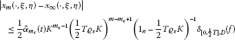
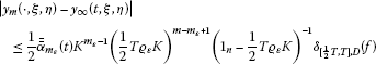
In order to prove a statement on the solvability of problem (1.3), (1.4), we need some estimates of the functions $Ξ m : G D (r D (f)) → R n$ and $H m : G D (r D (f)) → R n$ , $m = 0, 1, …$ , defined by (9.1) and (9.2).

Lemma 9.2 Assume that (6.20) holds. Let f satisfy the Lipschitz condition (1.5) with a matrix K such that

r (K) ≤ 20 3 T .

(9.7)

Then the estimates

| Ξ (ξ, η) − Ξ m (ξ, η) | ≤ 5 T 18 (320 T K) m + 1 (1 n − 320 T K) − 1 δ [0, 12 T], D (f)

(9.8)

and

| H (ξ, η) − H m (ξ, η) | ≤ 5 T 18 (320 T K) m + 1 (1 n − 320 T K) − 1 δ [12 T, T], D (f)

(9.9)

hold for any values of $(ξ, η) ∈ G D (r D (f))$ and $m ≥ 2$ .

Proof Let us fix arbitrary $(ξ, η) ∈ G D (r D (f))$ and $m ≥ 2$ . Recalling (6.10) and (9.1), we obtain

| Ξ (ξ, η) − Ξ m (ξ, η) | = | ∫ 0 T 2 [f (t, x ∞ (t, ξ, η)) − f (t, x m (t, ξ, η))] d t | ≤ ∫ 0 T 2 | f (t, x ∞ (t, ξ, η)) − f (t, x m (t, ξ, η)) | d t .

(9.10)

By Lemma 7.3, the function $x ∞ (⋅, ξ, η) : [0, 12 T] → R n$ has values in D and, therefore, the Lipschitz condition (1.5) can be used in (9.10). Then, applying estimate (6.11) of Theorem 6.1 with $ε = ε 0$ , where $ε 0 ≈ 0.00727$ is given by (3.14), we obtain

(9.11)

Recall now that, in view of Remark 6.2 and relations (3.11) and (3.14), one has

m ε 0 = 2, ϱ ε 0 = 310,

(9.12)

and, therefore, (9.11) can be rewritten in the form

(9.13)

Furthermore, it follows from (4.12) and (4.10) that the function $α ¯ 2$ has the form

α ¯ 2 (t) = (16 3 T 2 t 3 − 16 3 T t 2 + t + T 6) t, t ∈ [0, 12 T],

(9.14)

whence we obtain by computation that

∫ 0 T 2 α ¯ 2 (t) d t = T 3 80 .

(9.15)

Considering (9.12) and (9.15), we find that inequality (9.11), in fact, means that

| Ξ (ξ, η) − Ξ m (ξ, η) | ≤ T 3 160 K 2 (320 T K) m − 1 (1 n − 320 T K) − 1 δ [0, 12 T], D (f),

(9.16)

which estimate coincides with (9.8). Note that the invertibility of the matrix $1 n − 320 T K$ is guaranteed by condition (9.7).

In a similar manner, in order to establish (9.9), we use (6.17) and (9.1) to obtain the estimate

| H (ξ, η) − H m (ξ, η) | = | ∫ T 2 T [f (t, y ∞ (t, ξ, η)) − f (t, y m (t, ξ, η))] d t | ≤ ∫ T 2 T | f (t, y ∞ (t, ξ, η)) − f (t, y m (t, ξ, η)) | d t .

(9.17)

Lemma 7.3 guarantees that all the values of the function $y ∞ (⋅, ξ, η) : [12 T, T] → R n$ lie in D and, therefore, the Lipschitz condition (1.5) can be used in (9.17). Estimate (6.18) of Theorem 6.1 applied with $ε = ε 0$ then yields

(9.18)

Finally, it follows from (4.13) and (4.11) by computation that

α ¯ ¯ 1 (t) = 16 3 T 2 t 4 − 16 T t 3 + 17 t 2 − 15 T 2 t + 7 T 2 6, t ∈ [12 T, T],

(9.19)

and, hence,

∫ T 2 T α ¯ ¯ 2 (t) d t = T 3 80 .

(9.20)

Consequently, by virtue of relations (9.12) and (9.20), inequality (9.18) leads us directly to the required estimate (9.9). □

10 Solvability analysis based on approximation

The argument shown above allows us to conclude on the solvability of the periodic problem (1.3), (1.4) on the basis of properties of iterations (5.2) and (5.4). More precisely, it turns out that the use of functions (9.1) and (9.2) allows one to study the vector field $Φ : G D (r D (f)) → R 2 n$ ,

Φ (ξ, η) : = (η − ξ − ∫ 0 T 2 f (τ, x ∞ (τ, ξ, η)) d τ ξ − η − ∫ T 2 T f (τ, y ∞ (τ, ξ, η)) d τ), (ξ, η) ∈ G D (r D (f)),

(10.1)

the critical points of which, as we have seen in Theorem 8.1, determine the solutions of the original problem (1.3), (1.4), through its approximation

Φ m (ξ, η) : = (η − ξ − ∫ 0 T 2 f (τ, x m (τ, ξ, η)) d τ ξ − η − ∫ T 2 T f (τ, y m (τ, ξ, η)) d τ), (ξ, η) ∈ G D (r D (f)),

(10.2)

where m is fixed. In the formulation of the theorem given below, the following notion is used.

Definition 10.1 ([12])

Let r and l be positive integers and $S ⊂ R l$ be an arbitrary non-empty set. For any pair of vector functions $g j : R l → R r$ , $j = 1, 2$ , we write

g 1 ▷ S g 2

(10.3)

if and only if there exists a function $ν : S → {1, 2, …, l}$ such that the strict inequality

〈 g 1 (z) − g 2 (z), e ν (z) 〉 > 0

(10.4)

holds for all $z ∈ S$ .

Here, $e k$ , $k = 1, 2, …, r$ , are the unit vectors,

e k : = col (0, 0, …, 0 ⏟ k − 1, 1, 0, …, 0),

(10.5)

and $〈 ⋅, ⋅ 〉$ stands for the usual inner product in $R r$ . The binary relation $▷ S$ introduced by Definition 10.1 is a kind of strict inequality for vector functions and its properties are similar to those of the usual strict inequality sign. For example, $f ≥ g$ and $g ▷ S h$ imply that $f ▷ S h$ . The last named property will be used below in the proof of Theorem 10.2.

We are now able to formulate a statement guaranteeing the solvability of the original periodic problem (1.3), (1.4) based on the information obtained in the course of computation of iterations. In contrast to the unmodified scheme of periodic successive approximations (Proposition 3.1, $r (K) < T − 1 ϱ ∗ − 1$ ), here the iterations are proved to be convergent under the assumption that is twice as weak as in the former case (Theorem 6.5, $r (K) < 2 T − 1 ϱ ∗ − 1$ ). A similar observation can be made concerning the assumption on the domain D (see Corollary 6.7 and the remarks related to conditions (6.30) and (6.31)).

When stating the existence theorem, we restrict our consideration to a slightly weaker version of condition (6.4), where the value $ϱ ∗ ≈ 0.2927$ is replaced by 0.3, and thus neglect the gap ( $0, 0.00727 …$ ) for ε in estimates (6.11) and (6.18).

Theorem 10.2 Assume that the function f in (1.3) satisfies the Lipschitz condition (1.5) with a matrix K such that inequality (9.7) holds and, moreover, the set D has property (6.20). Moreover, let there exist a closed domain

Ω ⊂ G D (r D (f))

such that, for a certain fixed value of $m ≥ 2$ , the mapping $Φ m$ given by formula (10.2) satisfies the conditions

deg (Φ m, Ω) ≠ 0

(10.6)

and

| Φ m | ▷ ∂ Ω 5 T 18 (M m δ [0, 12 T], D (f) M m δ [12 T, T], D (f)),

(10.7)

where

M m : = (320 T K) m + 1 (1 n − 320 T K) − 1 .

(10.8)

Then there exist certain values $(ξ ∗, η ∗) ∈ Ω$ such that the function $u ∞ (⋅, ξ ∗, η ∗)$ is a solution of the periodic boundary value problem (1.3), (1.4).

Recall that the symbol $▷ ∂ Ω$ in (10.7) is understood in the sense of Definition 10.1. It should be noted that condition (10.7) involves the values of functions on the boundary of Ω only.

Proof We shall use the lemmata stated above. By analogy to [12, 24], we shall prove that the fields Φ and $Φ m$ are homotopic. It will be sufficient to consider the linear deformation

Q θ : = Φ m + θ (Φ − Φ m),

(10.9)

where $θ ∈ [0, 1]$ . Indeed, it is clear that $Q θ$ is a continuous mapping on ∂ Ω for every $θ ∈ [0, 1]$ and, furthermore,

Q 0 = Φ m, Q 1 = Φ .

(10.10)

Let us fix an arbitrary pair $(ξ, η) ∈ ∂ Ω$ . According to (10.1) and (10.2), we have

| Q θ (ξ, η) | = | Φ m (ξ, η) + θ [Φ (ξ, η) − Φ m (ξ, η)] | ≥ | Φ m (ξ, η) | − | Φ (ξ, η) − Φ m (ξ, η) | .

(10.11)

On the other hand, by Lemma 9.2, estimates (9.8) and (9.9) true. Using relations (9.8) and (9.9) in (10.11), we show that

| Q θ | ▷ ∂ Ω 0

and hence $Q θ$ does not vanish on ∂ Ω for any θ. Thus, Φ is homotopic to $Φ m$ . The property of invariance of degree under homotopy then yields

deg (Φ, Ω) = deg (Φ m, Ω);

and therefore, in view of (10.6), we conclude that $deg (Φ, Ω) ≠ 0$ . Consequently, there exist vectors $ξ ∗$ and $η ∗$ possessing the properties indicated, and it only remains to refer to Theorem 8.1. The theorem is proved. □

Note that Theorem 10.2 provides solvability conditions based upon properties of approximations starting from the second one inclusively. A similar statement allowing to use the zeroth and the first approximations can be obtained if we use [[12], Lemma 3.16] instead of Lemma 3.2. In that case, condition (10.7) of Theorem 10.2 is replaced, respectively, by the relations

| Φ 0 | ▷ ∂ Ω 5 T 2 108 (K (1 n − 320 T K) − 1 δ [0, 12 T], D (f) K (1 n − 320 T K) − 1 δ [12 T, T], D (f))

(10.12)

and

| Φ 1 | ▷ ∂ Ω T 3 144 (K 2 (1 n − 320 T K) − 1 δ [0, 12 T], D (f) K 2 (1 n − 320 T K) − 1 δ [12 T, T], D (f)) .

(10.13)

11 Approximation of a solution

The theorem proved in the preceding section can be complemented by the following natural observation. Let $(ξ ˆ, η ˆ) ∈ Ω$ be a root of the approximate determining system (9.3) for a certain m. Then the function

U m (t) : = u m (t, ξ ˆ, η ˆ), t ∈ [0, T],

(11.1)

defined according to (9.4) can be regarded as the m th approximation to a solution of the periodic problem (1.3), (1.4). This is justified by Proposition 9.1 and the estimates

| x ∞ (t, ξ ˆ, η ˆ) − U m (t) | ≤ 12 α ¯ 1 (t) (320 T K) m (1 n − 320 T K) − 1 δ [0, 12 T], D (f)

(11.2)

for $t ∈ [0, 12 T]$ and

| y ∞ (t, ξ ˆ, η ˆ) − U m (t) | ≤ 12 α ¯ 1 (t) (320 T K) m (1 n − 320 T K) − 1 δ [12 T, T], D (f)

(11.3)

for $t ∈ [12 T, T]$ , which, as is easy to see from (9.4), follow directly from Theorem 6.5. A uniform inequality, not given here, can be obtained by estimating the mapping $(ξ, η) ↦ u m (t, ξ, η)$ for any fixed $t ∈ [0, T]$ .

It is worth to emphasise the role of the unknown parameters whose values appearing in (11.1) are determined from equations (9.3): $ξ ˆ$ is an approximation of the initial value of the periodic solution and $η ˆ$ is that of its value at $12 T$ .

As regards the practical application of Theorem 10.2, it should be noted that, according to (10.2), the mapping $Φ m$ is known in an analytic form because it is determined solely by the m th iteration, which is already constructed at the moment. Of course, the degree in (10.6) is the Brouwer degree because all the vector fields are finite-dimensional. Likewise, all the terms in the right-hand side of inequality (10.7) are computed explicitly (e.g., by using computer algebra systems).

12 An example

Let us consider the scalar π-periodic boundary value problem

(12.1)

(12.2)

where $h (t) : = 12 (3 cos 2 t − sin 2 t) + 18 (sin 4 t + 1)$ , $t ∈ [0, π]$ . It is easy to check that the function

u (t) = 12 (cos 2 t + sin 2 t), t ∈ [0, π],

(12.3)

is a solution of problem (12.1), (12.2). This solution has values in the domain $D : = [− 1, 1]$ , where, as one can verify, the convergence condition (3.5) is not satisfied. However, the corresponding condition with the doubled constant (3.18) does hold, and therefore, the interval halving technique can be used.

The appropriate computations, which have been carried out by using Maple 14 and are omitted here, show that the approach based on Theorems 6.5 and 10.2 is indeed applicable in this case. The existence of solution (12.3) (let us forget for a moment that we know it explicitly in this academic example) is established by Theorem 10.2, whereas its approximations of type (11.1) are constructed as described above. For instance, in the first approximation, we have $u ≈ U 1$ with

U 1 (t) : = χ π (t) x 1 (t) + (1 − χ π (t)) y 1 (t), t ∈ [0, π],

where $χ π$ is the indicator function (4.5) and

x 1 (t) : = − 0.0266088895 + 0.7499999998 (cos t) 2 + 1.499999999 sin t cos t − 0.25 (cos t) 4 − 0.4392877052 t, t ∈ [0, 12 T],

(12.4)

and

y 1 (t) : = − 1.406671916 + 0.07499999995 (cos t) 2 − 0.25 (cos t) 4 + 1.5 sin t cos t + 0.4392877052 t, t ∈ [12 T, T] .

(12.5)

The numerical values of the parameters ξ and η corresponding to functions (12.4), (12.5) (see Table 1) are found from the system of equations (9.3) with $m = 1$ , which, in this case, have the form

and

Table 1 Approximate values of parameters at several steps of iteration for problem ( 12.1 ), ( 12.2 ). The last row corresponds to the exact solution ( 12.3 )

Full size table

The graphs obtained in the course of computation are shown on Figures 3 and 4, whereas Table 1 contains the corresponding numerical values of the parameters. Note that only the zeroth approximation has derivative with a discontinuity at $12 T$ (cf. Proposition 9.1). The graphs and the computed numerical values of the parameters show a rather good accuracy of approximation.

13 Comments

Several points can be outlined in relation to the techniques discussed in the preceding sections.

13.1 Approximation scheme in practice

An interesting feature of the approach indicated here is that a practical analysis of the periodic problem (1.3), (1.4) along its lines starts directly with the computation of iterations. We construct the approximate determining equations (9.3), solve them numerically in an appropriate region, substitute the corresponding roots into the formula for $u m$ and form functions (11.1) which are, in a sense, candidates for approximations of a solution. Having constructed functions (11.1) for several values of m, we check their behaviour heuristically and if it exhibits some signs of being possibly convergent, we stop the computation and verify the assumptions of the existence theorem. If successful, then, since this moment, we already know that a solution exists, and either we are satisfied with the achieved accuracy of approximation (in this case, the scheme stops and the function $U m$ given by (11.1) for the last computed value of m is proclaimed as its outcome) or, for some reasons, we find that a more accurate approximation is needed (one more step is made then, and a similar check is carried out for the new approximation).

It is important to observe that, once the existence of a solution is known from Theorem 10.2 at the m th step of iteration, we immediately obtain an approximation to it in the form (11.1). The scheme thus allows us to both study the solvability of the periodic problem and construct approximations to its solution.

It should be noted that the ability to derive the fact of solvability of the original problem from the corresponding properties of approximate problems is rather uncommon (see [12] for some details). For the numerical methods, the generic situation is, in fact, quite the reverse, when some or another technique is applied to solve a problem which is a priori assumed to be solvable.

13.2 Extension to other problems

The idea expressed above can easily be adopted for application to differential equations with argument deviations. The only issue that should be clarified in that case is the definition of iterations on the half-intervals at those points which are thrown over the middle to the adjacent half-interval. For this purpose, sequences (5.2) and (5.4) should be computed simultaneously, with (5.4) serving as an initial function for (5.2) at the next step, and vice versa.

Likewise, with appropriate modifications, the technique developed here can be applied to problems with boundary conditions other than periodic ones. We do not dwell on this topic here.

13.3 Variable subinterval lengths

It is, of course, not necessary to keep the $1 : 2$ ratio of subinterval lengths. For example, if there is a point $s 0$ such that $δ [0, s 0], D (f)$ is much greater than $δ [s 0, T], D (f)$ , the halving, or any other kind of division, is natural to be continued on $[0, s 0]$ . This reminds us of the idea used in the adaptive numerical methods with a variable step length.

13.4 Applicability on small intervals

In contrast to purely numerical approaches, where one may be forced to discretise with a tiny step, the efficiency of the technique based on Theorem 6.5 is not so much affected by the smallness of the interval. This makes the scheme well applicable, in particular, for the study of high-frequency oscillations.

13.5 Advantages over other methods

The proposed technique has some other positive features distinguishing it from other approaches. For example, when applying it, one experiences no difficulties with the selection of the starting approximation (in contrast, e.g., to monotone iterative methods); there is no need to re-calculate considerable amounts of data when passing to the next step of approximation (unlike projection methods); the global Lipschitz condition and the assumption on the unique solvability of the Cauchy problem are not necessary (unlike shooting method); etc. As regards the last mentioned condition, one should note that, for functional differential equations, it is violated even in very simple cases, and it is thus unnatural to require it when constructing a scheme of analysis of a reasonably wide class of problems.

13.6 Repeated interval halving

The interval halving procedure can be repeated. When doing so, we observe that conditions both on the eigenvalues of the Lipschitz matrix and the size of the domain are weakened by half at each step. Indeed, it follows immediately from Corollary 6.7 that the periodic successive approximation scheme constructed with k interval halvings is applicable provided that

r (K) < 2 k T ϱ ∗

(13.1)

and

D (T 2 k + 2 δ [0, T], D (f)) ≠ ∅ .

(13.2)

It is also clear that the $D (2 − k − 2 T δ [0, T], D (f))$ , $k = 0, 1, …$ , is a strictly increasing sequence of sets tending to the original domain D in the limit as k grows to ∞. In other words, rather interestingly, the scheme suggested here is theoretically applicable however large the eigenvalues of K may be.

The side-effect of the successive interval halving is the increase of the dimension of the system of determining equations, which contains $2 k n$ equations at the k th interval halving. One can regard this as a certain price to be paid for being able to apply interval halving in order to convert a divergent iteration scheme into a convergent one.

In this way, by carrying out interval halving sequentially, one can, in particular, re-establish the convergence of numerical-analytic algorithms for systems of ordinary differential equations with globally Lipschitzian non-linearities (see [12, 25, 26]).

13.7 Combination with other methods

The most difficult part of the scheme discussed consists in the analytic construction of so many members of the parametrised iteration sequence (9.4) which is sufficient to establish the solvability of the periodic problem (see conditions (10.6), (10.7)) and achieve the required precision of approximation in (11.1). Its practical implementation, usually done by using symbolic computation systems, can be considerably facilitated by combining the analytic computation with a suitable kind of approximation. The use of the polynomial or trigonometric interpolation (see [10, 27]) is very convenient for this purpose.

13.8 Non-degeneracy condition for higher-order approximations

It is obvious from (9.7) and (10.8) that $lim m → ∞ M m = 0$ and, hence, the right-hand side of inequality (10.7) vanishes when m grows to +∞. On the other hand, it is easy to see that, under the conditions assumed, the mapping $Φ m$ (uniformly on compact sets) converges to Φ as m tends to +∞. We thus arrive at the interesting observation that assumption (10.7) of Theorem 10.2, which is the main condition ensuring the non-degeneracy of the homotopy, has the form of the strict inequality

| Φ m | ▷ ∂ Ω w m,

where $| Φ m |$ approaches to $| Φ |$ while the term $w m$ becomes arbitrarily small as m grows to +∞.

13.9 Relation to continuation theorems

Theorem 10.2 and similar statements can also be applied on the zeroth step of iteration, i.e., when one does not perform any iteration at all. This reminds us of the notion of a generating system appearing, e.g., in the asymptotic methods.

Indeed, having in mind Theorem 10.2 in its present formulation and recalling condition (10.12), let us put

f # (ξ, η) : = (η − ξ − ∫ 0 T 2 f (τ, (1 − 2 t T) ξ + 2 t T η) d τ ξ − η − ∫ T 2 T f (τ, (2 t T − 1) ξ + 2 (1 − t T) η) d τ)

(13.3)

for any $(ξ, η) ∈ G D (r D (f))$ . Recall that $G D (r D (r))$ is a subset of $D 2$ which a priori contains the value $(u (0), u (12 T))$ for the periodic solution $u (⋅)$ in question.

By using Theorem 10.2 for $m = 0$ with condition (10.7) replaced by (10.12), we obtain the following statement on the solvability of the periodic problem (1.3), (1.4).

Corollary 13.1 Let assumption (6.20) hold and let the convergence condition (9.7) be satisfied. Furthermore, let there exist a closed domain $Ω ⊂ G D (r D (f))$ such that

deg (f #, Ω) ≠ 0

(13.4)

and

| f # | ▷ ∂ Ω 5 T 2 108 (K (1 n − 320 T K) − 1 δ [0, 12 T], D (f) K (1 n − 320 T K) − 1 δ [12 T, T], D (f)) .

(13.5)

Then the periodic boundary value problem (1.3), (1.4) has at least one solution $u (⋅)$ which has values in D and, moreover, is such that $(u (0), u (12 T)) ∈ Ω$ .

Recall that the vectors $δ [0, 12 T], D (f)$ and $δ [12 T, T], D (f)$ are computed directly according to formula (2.1), whereas ‘ $▷ ∂ Ω$ ’ means that, at every point from ∂ Ω, the strict inequality ‘>’ holds for at least one row, and the number of that row may vary with the point.

Assumptions of type (6.12), (13.5) are natural from various points of view. For example, let us imagine for a while that no interval halving has been carried out at all and thus, instead of Theorem 6.5, we are in the situation described by Proposition 3.1 with $g = f$ , $p = T$ and $t 0 = 0$ . The system of 2n determining equations (8.2) then turns back into the n-dimensional system (3.15),

∫ 0 T f (t, u ∞ (t, ξ)) d t = 0,

the zeroth approximation of which, in the sense of the iteration process (3.4), has the form

∫ 0 T f (t, ξ) d t = 0 .

(13.6)

Therefore, assumption (6.12) becomes

deg (f ¯, V) ≠ 0

(13.7)

with a suitable domain $V ⊂ D$ , where

f ¯ (ξ) : = ∫ 0 T f (t, ξ) d t

(13.8)

for $ξ ∈ V$ . Then, using [[12], Lemma 3.26] with $m = 0$ , one easily shows that the following statement holds.

Corollary 13.2 The conditions (13.7), $r (K) < 10 (3 T) − 1$ and

| f ¯ | ▷ ∂ V 5 T 2 27 K (1 n − 310 T K) − 1 δ [0, T], D (f)

(13.9)

are sufficient for the solvability of the periodic problem (1.3), (1.4).

Arguing in this manner, we can obtain, in particular, the well-known Mawhin’s theorem [28], with (13.7) being the solvability condition for the generating equation (of course, one could use the condition of a priori bounds type instead of (13.9) for a more exact resemblance). In this context, Corollary 13.1 can be regarded as a ‘halved’ analogue of the last mentioned statement, where the equations

(13.10)

(13.11)

determine the initial data of the zeroth approximation. The side-effect of halving is visible from the presence of two independent variables, ξ and η, due to which system (13.10), (13.11), in contrast to (13.6), contains n extra equations.

It should be noted that the convergence of the iteration scheme in Corollary 13.1 is guaranteed under the assumption $r (K) < 20 (3 T) − 1$ , which is twice as weak as the corresponding condition of Corollary 13.2 ( $r (K) < 10 (3 T) − 1$ ).

References

1.
Rontó A, Rontó M: Periodic successive approximations and interval halving. Miskolc Math. Notes 2012, 13(2):459-482.
MATH MathSciNet Google Scholar
2.
Nirenberg L: Topics in Nonlinear Functional Analysis. Courant Institute of Mathematical Sciences New York University, New York; 1974. (With a chapter by E. Zehnder, Notes by R. A. Artino, Lecture Notes, 1973-1974)
Google Scholar
3.
Gaines RE, Mawhin JL Lecture Notes in Mathematics 568. In Coincidence Degree, and Nonlinear Differential Equations. Springer, Berlin; 1977.
Google Scholar
4.
Cesari L Ergebnisse der Mathematik und Ihrer Grenzgebiete, N. F. 16. In Asymptotic Behavior and Stability Problems in Ordinary Differential Equations. 2nd edition. Academic Press, New York; 1963.
Google Scholar
5.
Hale JK: Oscillations in Nonlinear Systems. McGraw-Hill, New York; 1963.
Google Scholar
6.
Samoilenko AM: A numerical-analytic method for investigation of periodic systems of ordinary differential equations. I. Ukr. Math. J. 1965, 17(4):82-93. 10.1007/BF02526569
Article Google Scholar
7.
Samoilenko AM: A numerical-analytic method for investigation of periodic systems of ordinary differential equations. II. Ukr. Math. J. 1966, 18(2):50-59. 10.1007/BF02537778
Article Google Scholar
8.
Samoilenko AM: On a sequence of polynomials and the radius of convergence of its Abel-Poisson sum. Ukr. Math. J. 2003, 55(7):1119-1130. doi:10.1023/B:UKMA.0000010610.69570.13
Article Google Scholar
9.
Samoilenko AM, Ronto NI: Numerical-Analytic Methods of Investigating Periodic Solutions. Mir, Moscow; 1979. (With a foreword by Yu. A. Mitropolskii)
Google Scholar
10.
Samoilenko AM, Ronto NI: Numerical-Analytic Methods of Investigation of Boundary-Value Problems. Naukova Dumka, Kiev; 1986. (In Russian, with an English summary, edited and with a preface by Yu. A. Mitropolskii)
Google Scholar
11.
Samoilenko AM, Ronto NI: Numerical-Analytic Methods in the Theory of Boundary-Value Problems for Ordinary Differential Equations. Naukova Dumka, Kiev; 1992. (In Russian, edited and with a preface by Yu. A. Mitropolskii)
Google Scholar
12.
Rontó A, Rontó M: Successive approximation techniques in non-linear boundary value problems for ordinary differential equations. Handb. Differ. Equ. In Handbook of Differential Equations: Ordinary Differential Equations. Vol. IV. Elsevier/North-Holland, Amsterdam; 2008:441-592.
Google Scholar
13.
Rontó A, Rontó M: Successive approximation method for some linear boundary value problems for differential equations with a special type of argument deviation. Miskolc Math. Notes 2009, 10: 69-95.
MATH MathSciNet Google Scholar
14.
Rontó A, Rontó M: On a Cauchy-Nicoletti type three-point boundary value problem for linear differential equations with argument deviations. Miskolc Math. Notes 2009, 10(2):173-205.
MATH MathSciNet Google Scholar
15.
Rontó A, Rontó M: On nonseparated three-point boundary value problems for linear functional differential equations. Abstr. Appl. Anal. 2011., 2011: Article ID 326052. doi:10.1155/2011/326052
Google Scholar
16.
Ronto A, Rontó M: A note on the numerical-analytic method for nonlinear two-point boundary-value problems. Nonlinear Oscil. 2001, 4: 112-128.
MATH MathSciNet Google Scholar
17.
Rontó A, Rontó M: On some symmetric properties of periodic solutions. Nonlinear Oscil. 2003, 6: 82-107. doi:10.1023/A:1024827821289 10.1023/A:1024827821289
MathSciNet Article Google Scholar
18.
Rontó M, Shchobak N: On the numerical-analytic investigation of parametrized problems with nonlinear boundary conditions. Nonlinear Oscil. 2003, 6(4):469-496. doi:10.1023/B:NONO.0000028586.11256.d7
MathSciNet Article Google Scholar
19.
Rontó M, Shchobak N: On parametrization for a non-linear boundary value problem with separated conditions. Electron. J. Qual. Theory Differ. Equ. 2007, 18: 1-16.
Article Google Scholar
20.
Ronto AN, Ronto M, Shchobak NM: On the parametrization of three-point nonlinear boundary value problems. Nonlinear Oscil. 2004, 7(3):384-402. 10.1007/s11072-005-0019-5
MathSciNet Article Google Scholar
21.
Ronto AN, Rontó M, Samoilenko AM, Trofimchuk SI: On periodic solutions of autonomous difference equations. Georgian Math. J. 2001, 8: 135-164.
MATH MathSciNet Google Scholar
22.
Rontó M, Mészáros J: Some remarks on the convergence of the numerical-analytical method of successive approximations. Ukr. Math. J. 1996, 48: 101-107. doi:10.1007/BF02390987 10.1007/BF02390987
MATH Article Google Scholar
23.
Rontó M, Samoilenko AM: Numerical-Analytic Methods in the Theory of Boundary-Value Problems. World Scientific, River Edge; 2000. (With a preface by Yu. A. Mitropolsky and an appendix by the authors and S. I. Trofimchuk)
Google Scholar
24.
Rontó A, Rontó M: Existence results for three-point boundary value problems for systems of linear functional differential equations. Carpath. J. Math. 2012, 28: 163-182.
MATH Google Scholar
25.
Kwapisz M: On modifications of the integral equation of Samoilenko’s numerical-analytic method of solving boundary value problems. Math. Nachr. 1992, 157: 125-135.
MATH MathSciNet Google Scholar
26.
Kwapisz M: On modification of Samoilenko’s numerical-analytic method of solving boundary value problems for difference equations. Appl. Math. 1993, 38(2):133-144.
MATH MathSciNet Google Scholar
27.
Rontó A, Rontó M, Holubová G, Nečesal P: Numerical-analytic technique for investigation of solutions of some nonlinear equations with Dirichlet conditions. Bound. Value Probl. 2011., 2011: Article ID 58. doi:10.1186/1687-2770-2011-58
Google Scholar
28.
Mawhin J CBMS Regional Conference Series in Mathematics 40. In Topological Degree Methods in Nonlinear Boundary Value Problems. Am. Math. Soc., Providence; 1979. (Expository lectures from the CBMS Regional Conference held at Harvey Mudd College, Claremont, Calif., June 9-15, 1977)
Google Scholar

Download references

Acknowledgements

Dedicated to Professor Jean Mawhin on the occasion of his 70th birthday.

The work supported in part by RVO: 67985840 (A. Rontó). This research was carried out as part of the TAMOP-4.2.1.B-10/2/KONV-2010-0001 project with support from the European Union, co-financed by the European Social Fund (M. Rontó).

Author information

Affiliations

Institute of Mathematics, Academy of Sciences of Czech Republic, 22 Žižkova St., Brno, 616 62, Czech Republic
András Rontó
Department of Analysis, University of Miskolc, Egyetemváros, Miskolc, 3515, Hungary
Miklós Rontó
Uzhgorod National University, 46 Pidhirna St., Uzhgorod, 88000, Ukraine
Nataliya Shchobak

Authors

András Rontó
View author publications
You can also search for this author in PubMed Google Scholar
Miklós Rontó
View author publications
You can also search for this author in PubMed Google Scholar
Nataliya Shchobak
View author publications
You can also search for this author in PubMed Google Scholar

Corresponding author

Correspondence to András Rontó.

Additional information

Competing interests

The authors declare that they have no competing interests.

Authors’ contributions

The initial draft was prepared mainly by the first two authors, while the third one carried out the numerical computations and an overall check of estimates. All the authors contributed equally to the final version of this work and approved its present form.

Authors’ original submitted files for images

Below are the links to the authors’ original submitted files for images.

Authors’ original file for figure 1

Authors’ original file for figure 2

Authors’ original file for figure 3

Authors’ original file for figure 4

Rights and permissions

Open Access This article is distributed under the terms of the Creative Commons Attribution 2.0 International License (https://creativecommons.org/licenses/by/2.0), which permits unrestricted use, distribution, and reproduction in any medium, provided the original work is properly cited.

Reprints and Permissions

About this article

Cite this article

Rontó, A., Rontó, M. & Shchobak, N. Constructive analysis of periodic solutions with interval halving. Bound Value Probl 2013, 57 (2013). https://doi.org/10.1186/1687-2770-2013-57

Download citation

Received: 27 December 2012
Accepted: 28 February 2013
Published: 22 March 2013
DOI: https://doi.org/10.1186/1687-2770-2013-57

Keywords

periodic solution
periodic boundary value problem
parametrisation
periodic successive approximations
numerical-analytic method
interval halving
existence
continuation
Mawhin’s theorem