- Research
- Open access
- Published:
The solutions for the flow of micropolar fluid through an expanding or contracting channel with porous walls
Boundary Value Problems volume 2016, Article number: 176 (2016)
Abstract
The unsteady, two-dimensional laminar flow of an incompressible micropolar fluid in a channel with expanding or contracting porous walls is investigated. The governing equations are transformed into a coupled nonlinear two-points boundary value problem by a suitable similarity transformation. Unlike the classic Berman problem (Berman in J. Appl. Phys. 24:1232-1235, 1953), three new solutions (totally six solutions) and no-solution interval, which is one of important characteristics for the laminar flow through porous pipe with stationary wall (Terrill and Thomas in Appl. Sci. Res. 21:37-67, 1969), are found numerically for the first time. The multiplicity of the solutions is strictly dependent on the expansion ratio. Furthermore, the asymptotic solutions are constructed by the Lighthill method, which eliminates the singularity of the similarity solution, for large injection and by the matching theorem for the suction Reynolds number, respectively. The analytical solutions also are compared with the numerical ones and the results agree well.
1 Introduction
The studies of laminar flow in an expanding or contracting channel or pipe with permeable wall have received considerable attentions due to its application in biophysical flows in recent years. The pioneering work may have been done by Uchida and Aoki [3] to simulate the successive peristaltic motion of the artery, who examined the viscous flow inside an impermeable tube with a contracting cross section. Later, Goto and Uchida [4] analyzed the incompressible laminar flow in a semi-infinite porous pipe whose radius varied with time. In addition, further experiments carried out by Wilens [5], Evans et al. [6], and Michel [7] proved the endothelial walls to be permeable with ultra-microscopic pores, through which the mass transfer takes place between blood, air, and tissue. It has also been pointed out that the deposition of cholesterol and the dilated damaged and inflamed arterial walls may cause an increase in its permeability. Recently, Majdalani et al. [8–10] investigated the flow of the fluid through an expanding channel with porous walls by numerical or asymptotical methods and analyzed the influence of the permeability and the expansion ratio on the velocity and pressure distribution.
In general, blood flow is regarded as a non-Newtonian fluid through a pipe or channel. The rheological properties of the blood are mainly due to the suspension of red blood cells, white cells, and platelets in the blood plasma. These properties strongly affect the dynamics of blood flow and render blood a non-Newtonian fluid [11]. The theory of micopolar fluids proposed by Eringen [12, 13] is one of the best theories of fluids to describe the deformation of such materials. Physically these fluids may represent the fluids consisting of rigid randomly oriented particles suspended in a viscous medium undergoing both translational and rotational motion. Furthermore, experimental studies have revealed that the blood’s viscosity decreases with the increase in shear rate, and that blood has a small yield stress. Airman et al. [14, 15] made excellent reviews about the applications of micropolar fluids. Pazanin [16] presented the result as regards an asymptotic approximation of the micropolar fluid flow through a thin or long straight pipe with variable cross section and explicitly addressed the effects of the microstructure on the flow. Ziabakhsh and Domairry [17] and Joneidi et al. [18] discussed the micropolar fluid in a porous channel by a homotopy analysis method (HAM). Ramachandran et al. [19] studied the heat transfer of a micropolar fluid past a curved surface with suction and injection using Van Dyke’s singular perturbation technique. Si et al. [20] investigated the mass and heat transfer of the micropolar fluid through an expanding channel with porous walls by HAM and analyzed the effects of the heat dissipation on the velocity and temperature distribution.
Apart from the above work, solution multiplicity is a classic problem for the equations describing the flow in channels or pipes with porous walls. A similar problem has been studied by Berman [1] and Terrill [21], who assumed that the wall is stationary. The multiplicity of the solutions has been addressed by Terrill [21], Terrill and Thomas [2], Robinson [22], MacGillivray and Lu [23], Lu et al. [24], and Zaturska et al. [25]. More recently, a theoretical treatment was done by Xu et al. [26], who revisited the Newtonian fluid in the channel with porous orthogonally moving walls by homotopy analysis method (HAM), and the results have shown that there exist dual or triple solutions corresponding to the cases reported by Zaturska et al. [25]. Almost at the same time, Si et al. [27, 28] also obtained the dual solutions of the flow in the expanding pipe and channel with porous walls, where they consider the small expansion ratio and large suction Reynolds number by singular perturbation methods. In addition, some other similar numerical and experimental studies also have been reported on multiple solutions. For example, Luo and Pedley [29] investigated two-dimensional limitation flow in a collapsible channel and multiple steady solutions were found for a range of physical parameters. Siviglia and Toffolon [30] discussed one-dimensional flow through a collapsible tube and found that geometrical alterations or variations of the mechanical properties of the tube wall affected the occurrence of multiple flow states. Lanzerstorfer and Kuhlmann [31] studied numerically the global stability of multiple solutions for the flow in a sudden expansion plane. Putkaradze and Vorobieff [32] made some experiments to show the multiple solutions of the flow in an expanding channel.
Motivated by the above-mentioned studies, the aim of this paper is to investigate the flow of an incompressible micropolar fluid in a channel with deforming porous walls. The paper is organized as follows. In Section 2 we introduce the laminar flow equations and the similarity transformation which reduce the governing equations to a system of high order nonlinear ordinary differential ones. In Section 3 we discuss the characteristics of different types of solution obtained by Bvp4c, which is a collocation method equivalent to the fourth order monoimplicit-Runge-Kutta method. In Section 4 we construct the asymptotic solutions with large injection or suction velocity, which are compared with the numerical ones obtained in Section 3. In Section 5 the conclusion is drawn.
2 Governing equations
We consider the unsteady, incompressible, laminar flow of a micropolar fluid in a semi-infinite channel with porous walls. The distance \(2a(t)\) between the walls is much smaller than the width and length of the channel. One end of the channel is closed by a complicated solid membrane. Both walls have equal permeability \(v_{w}\) and expand or contract uniformly in the transverse direction at a time-dependent rate \(\dot{a}(t)\). As shown in Figure 1, a coordinate system is chosen with the origin at the center of the channel. Take x and y to be coordinate axes parallel and perpendicular to the channel walls, respectively.

The model of the porous channel with expanding or contracting walls.
The governing equations of the flow are expressed as follows [18, 20]:
where u, v is the velocity components in the x and y directions and N is the microrotation, respectively. ρ, p, μ, κ, j, and γ are the density, pressure, dynamic viscosity, vortex viscosity coefficient, micro-inertia, and the spin gradient viscosity coefficient, respectively. Here γ is assumed to be [33]
The corresponding boundary conditions are [8, 20]
where A is the injection coefficient, which is a measure of the wall permeability.
Motivated by the definition of the stream function [8, 20], in this paper we define
Substituting equation (8) into equations (1), (2), (3), (4), one obtains the following equations:
where \(\alpha=\frac{a\dot{a}}{\upsilon}\) is the expansion ratio, and \(K=\frac{\kappa}{\mu}\) and \(N_{1}=\frac{\kappa a^{2}}{j\mu}\) are micropolar parameters. In accordance with the physical meaning, the positive α represents the expanding walls.
The boundary conditions become
where \(\mathit{Re}=\frac{a v_{w}}{\upsilon}\) is the permeability Reynolds number.
A similar solution with respect to both space and time can be developed following the transformation described by Uchida and Aoki [4], Dauenhauer and Majdalani [10], and Si et al. [20], respectively. This can be accomplished by considering the case: α is a constant, and \(F_{\eta\eta t}=0\) and \(G_{t}=0\). Similar to [10], the normal pressure gradient and axial pressure gradient can be obtained by substituting equation (8) into equations (2) and (3), which are listed as follows:
and
Equations (9), (10), (11), (12) can be normalized by the following transformations:
and so
The boundary conditions become
In physical meaning, this model is based on a decelerating wall dilation rate that follows a plausible assumption [3, 10]:
where \(a_{0}\) and \(\dot{a}_{0}\) are the initial height and expansion rate of the channel. Then the expressions for the height and velocity at time t of the wall can be obtained,
3 Numerical results and discussions
As mentioned before, multiple solutions associated with fluid mechanics have been attracted many researchers’ attention. Recently, Yao [34] claimed that the Reynolds number is insufficient to determine a flow field uniquely for a given geometry. The non-uniqueness of fluid flow means that the different frequencies of flows can exist on each stable bifurcation branch. Here the multiple solutions are obtained numerically by Bvp4c [35] and we set the maximum residual error as 10−4 during the computation.
Compared with the classic works obtained by Robinson [22], MacGillivray and Lu [23], Zaturska et al. [25], which are related with the Newtonian flow with stationary porous walls, the numerical solutions obtained by us lead to the new conclusions:
-
(i)
As is shown in Figures 2, 3, 4, the solutions of types I, II, III exist for all the values of the expansion ratio. In addition, the interval of existence for the solutions types II, III varies with the expansion ratio.
Figure 2 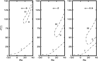
The effects of the negative expansion ratio α on the solutions as \(\pmb{K=0.1}\) , \(\pmb{N_{1}=0.1}\) .
Figure 3 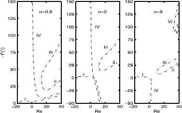
The effects of the positive expansion ratio α on the solutions as \(\pmb{K=0.1}\) , \(\pmb{N_{1}=0.1}\) .
Figure 4 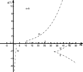
Axial velocity for type IV as \(\pmb{K=0.1}\) and \(\pmb{N_{1}=0.1}\) .
-
(ii)
The positive expansion ratio leads to the appearance of new types of solutions, which are illustrated in Figures 5-7. However, these solutions do not exist for every value of the expansion ratio.
Figure 5 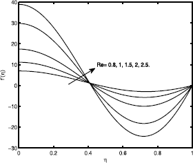
Axial velocity for type IV as \(\pmb{K=0.1}\) , \(\pmb{\alpha=5}\) , and \(\pmb{N_{1}=0.1}\) .
Figure 6 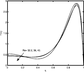
Axial velocity for type V as \(\pmb{K=0.1}\) , \(\pmb{\alpha=5}\) , and \(\pmb{N_{1}=0.1}\) .
Figure 7 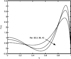
Axial velocity for type VI as \(\pmb{K=0.1}\) , \(\pmb{\alpha=5}\) , and \(\pmb{N_{1}=0.1}\) .
-
(iii)
For some values of the positive expansion ratio (i.e. \(\alpha=5\)), the interval \((2.72,9.77)\) of no solution appears. This phenomenon is similar to the case of the Newtonian flow through a stationary pipe with porous wall.
-
(iv)
The micropolar parameter has influence on the solutions, but it does not lead to the appearance of the new types of solutions, which is shown in Figures 8, 9.
Figure 8 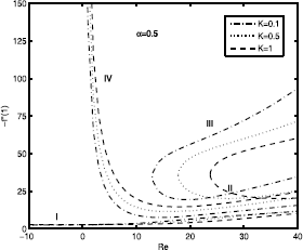
The effects of K on solutions as \(\pmb{\alpha=0.5}\) , \(\pmb{N_{1}=0.1}\) .
Figure 9 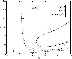
The effects of \(\pmb{N_{1}}\) on solutions as \(\pmb{\alpha=0.5}\) , \(\pmb{K=0.1}\) .


4 Perturbation analysis for this problem
4.1 Solution for the large injection Reynolds number
The singularity is due to large blowing at each wall which pushes the shear layer to the core region [36]. In order to eliminate the singular behavior, we employ the Lighthill method to obtain the asymptotic solution which is valid to arbitrary order as regards the derivative of the axial velocity.
One treats \(\varepsilon=1/\mathit{Re}\) as the perturbation parameter, then equations (16), (17) become
where λ is an integer constant. First of all, we introduce a variable transformation of η,
where the functions \(X_{1}\), \(X_{2}\) will be determined next.
Assume the function f, g, and the constant λ can be expanded in the following forms:
Substituting (25) into (22), (23), and collecting the same powers of ε, one can obtain the leading order of the solution
and the first order of the solution
Here the overdot \(\dot{\hphantom{a}}\) denotes the derivation with respect to ξ.
4.1.1 A. The transformed boundary condition at the wall
We assume ξ̃ is the root of (24) at \(\eta=1\), then
thus the condition at the wall can be obtained
Hence, the boundary conditions of \(f_{i}\) and \(g_{i}\) at \(\eta=1\) are
4.1.2 B. The transformed boundary condition at the core
One supposes that ξ̂ is the root of (24) at \(\eta=0\), then
thus we can induce
Hence, the boundary conditions of \(f_{i}\) and \(g_{i}\) at \(\eta=0\) are
Using (40), (41), and (42), the solution for (26) can be obtained,
and then \(\lambda_{0}=\frac{\pi^{2}}{4}\).
Substituting the above results into (27), (28) yields the following equations for \(f_{1}\), \(g_{1}\):
and
It is noted that using the method of variation of parameters to solve equation (44) will cause a singularity term in the solution [36]. In order to eliminate the singularity and to obtain \(f_{1}\), we can set
then we have
Thus, the equation for \(f_{1}\) becomes
whose solution is
where \(K_{1}\), \(K_{2}\) can be determined by boundary conditions, and the results are \(K_{1}=\frac{\pi}{2}C_{1}\), \(K_{2}=0\), \(\lambda_{1}=\alpha-\frac{(1+K)\pi^{2}}{4}\). For obtaining the nontrivial solution of \(f_{1}\), we set \(C_{1} = 1\). Thus, one can obtain \(f_{1}\), \(g_{1}\):
and
Finally, we obtain the asymptotic solution of f, g in terms of ξ as follows:
where
Tables 1 and 2 give the comparison between the asymptotic results of \(-f''(1)\), \(g'(1)\) with the numerical ones and the results agree well. The axial velocity and microrotation velocity profiles are showed in Figures 10, 11.

The effects of the expansion ratio α on the axial velocity as \(\pmb{\mathit{Re}=-100}\) , \(\pmb{K=0.1}\) , \(\pmb{N_{1}=0.1}\) .

The effects of the expansion ratio α on microrotation as \(\pmb{\mathit{Re}=-100}\) , \(\pmb{K=0.1}\) , \(\pmb{N_{1}=0.1}\) .
4.2 Solution for large suction Reynolds number
In order to capture an analytical solution satisfying all the boundary conditions and valid in the whole channel, the method of matched asymptotic expansion are used. Then equations (16), (17) can be written as
where k is a constant of integration. Here
where the coefficients \(\beta_{i}\), \(\sigma_{i}\), and \(\delta_{i}\) are constants determined by matching with the inner solutions. We assume that the forms of the outer solution are
Substituting (60) into (55), (56) and equating the same power of the coefficient ε, one obtains
The corresponding boundary conditions for the outer solutions are
According to the boundary conditions (69), it is not difficult to find the solutions of (61), (62),
then \(\sigma_{0}=f_{0}'''(0)=0\), \(\delta_{0}=g_{0}'(0)=\omega_{0}\).
Substituting (70) into (63), one obtains
then the solution of (71) satisfying the boundary conditions (69) is
where \(C_{1}\) is an integration constant, which will be determined next.
Substituting (70), (72) into (64), one obtains
then the solution of (73) satisfying the boundary conditions (69) is
Because \(g_{1}\) means the microrotation velocity of particles, \(g'_{1}(0)\rightarrow\infty\) leads to \(\omega_{0}=0\). Then
Substituting (70), (72), (75) into (65), one obtains
where \(C_{2}\) is an integration constant. Similarly, \(f'''_{2}(0)\rightarrow\infty\) leads to \(C_{1}=0\), \(\sigma_{1}=f_{1}'''(0)=0\), thus
and then \(\delta_{1}=g_{1}'(0)=\omega_{1}\), which will be determined in the next section.
In order to obtain the inner solution in the viscous layer, we introduce the stretching transformation \(\tau=(1-\eta)/\varepsilon\). Then (16) can be written as
Here the overdot denotes the derivative with respect to τ. According to the boundary conditions (19), we assume the inner solutions near the wall to be
Substituting (80) into (78), (79) yields the following equations:
The boundary conditions corresponding to the inner solution are
The solution of (81) is
where \(A_{0}=\frac{1}{1+K}\). Then the first two inner solution of f can be expressed as
The outer solution of f expressed in terms of the inner variable τ is
As \(\tau\rightarrow\infty\), matching the inner solution (87) with the outer solution (88) gives
The solution of (82) is
where \(B_{0}=\frac{2}{2+K}\) and \(\Omega_{1}\) will be determined in the following matching process. Then the first two inner solution of g can be expressed as follows:
The outer solution of g expressed in terms of the inner variable τ is
As \(\tau\rightarrow\infty\), matching the inner solution (91) with the outer solution (92) gives
According to (66), one can obtain
Then we obtain \(f_{3}\),
Similarly, \(f'''_{3}(0)\rightarrow\infty\) leads to \(C_{2}=0\), \(\sigma_{2}=f_{2}'''(0)=0\), thus
then
and from (83), one can obtain
As \(\tau\rightarrow\infty\), matching the inner and outer solution, one obtains
Then we obtain \(g_{3}\),
thus \(g'_{3}(0)\rightarrow\infty\) leads to \(\omega_{2}=0\). From (84), we obtain
then \(\delta_{2}=g'_{2}(0)=-\frac{2(K+1)(7K+10)N_{1}}{(K+2)(3K+4)}\).
Similarly, the comparison between the asymptotic and numerical solutions for different Reynolds numbers and expansion ratios is given in Tables 3 and 4. The axial velocity profiles and microrotation velocity profiles are presented in Figures 12, 13, and the results agree well.

The axial velocity as \(\pmb{\mathit{Re}=100}\) , \(\pmb{K=0.1}\) , \(\pmb{\alpha=5}\) , \(\pmb{N_{1}=0.1}\) .

The microrotation as \(\pmb{\mathit{Re}=100}\) , \(\pmb{K=0.1}\) , \(\pmb{\alpha=5}\) , \(\pmb{N_{1}=0.1}\) .
5 Conclusions
The micropolar fluid through a deforming channel with porous walls is investigated numerically and analytically. In addition, the perturbation solutions are constructed for large injection and suction permeability Reynolds number. Some conclusions can be drawn:
-
(i)
The multiplicity of the solutions is influenced by the Reynolds number and the expansion ratio of the channel. New types of solutions are captured when the walls are expanding. Moreover, the non-existence of solutions for a specified range of Reynolds numbers with a particular positive expanding ratio is discovered.
-
(ii)
In order to eliminate the singularity of the solution for the case of large injection, the analytical solution is constructed by the Lighthill method.
-
(iii)
For the case of a large suction, the matched asymptotic expansion is used to obtain the analytical solution by the matching of the inner solution with the outer solution.
In this paper, we only construct two solutions for large injection or suction Reynolds number by singular perturbation methods. Some other multiple asymptotic solutions may be constructed to complement the above results in the future, which will help us to better understanding the stability of the micropolar flow through a deforming channel with porous walls.
References
Berman, AS: Laminar flow in channels with porous walls. J. Appl. Phys. 24, 1232-1235 (1953)
Terrill, RM, Thomas, PW: Laminar flow in a uniformly porous pipe. Appl. Sci. Res. 21, 37-67 (1969)
Uchida, S, Aoki, H: Unsteady flows in a semi-infinite contracting or expanding pipe. J. Fluid Mech. 82, 371-387 (1977)
Goto, M, Uchida, S: Unsteady flows in a semi-infinite expanding pipe with injection through wall. Trans. Jpn. Soc. Aeronaut. Space Sci. 33(9), 14-27 (1990)
Wilens, SL: The experimental production of lipid deposition in excised arteries. Science 114, 389-393 (1951)
Evans, SM, Ihrig, HK, Means, JA, Zeit, W, Haushalter, ER: Atherosclerosis: an in vitro study of the pathogenesis of atherosclerosis. Am. J. Clin. Pathol. 22, 354-363 (1952)
Michel, CC: Direct observations of sites of permeability for ions and small molecules in mesothelium and endothelium. In: Capillary Permeability, pp. 628-642 (1970)
Majdalani, J, Zhou, C: Moderate-to-large injection and suction driven channel flows with expanding and contracting walls. Z. Angew. Math. Mech. 83, 181-196 (2003)
Majdalani, J, Zhou, C: Large injection and suction driven channel flows with expanding and contracting walls. In: 31st AIAA Fluid Dynamics Conference, Anaheim, CA, 11-14 June (2001)
Dauenhauer, CE, Majdalani, J: Exact self-similarity solution of the Navier-Stokes equations for a porous channel with orthogonally moving walls. Phys. Fluids 15, 1485-1495 (2003)
Silber, G, Trostel, R, Alizadeh, M, Benderoth, G: A continuum mechanical gradient theory with applications to fluid mechanics. J. Phys. 8, 365-373 (1998)
Eringen, AC: Theory of micropolar fluids. J. Math. Mech. 16, 1-18 (1966)
Eringen, AC: Theory of thermomicropolar fluids. J. Math. Anal. Appl. 38, 480-496 (1972)
Ariman, T, Turk, MA, Sylvester, ND: Microcontinuum fluid mechanics - a review. Int. J. Eng. Sci. 11, 905-930 (1973)
Ariman, T, Turk, MA, Sylvester, ND: Applications of microcontinuum fluid mechanics. Int. J. Eng. Sci. 12, 273-293 (1974)
Pazanin, I: Effective flow of micropolar fluid through a thin or long pipe. Math. Probl. Eng. 2011, Article ID 127070 (2011)
Ziabakhsh, Z, Domairry, G: Homotopy analysis solution of micro-polar flow in a porous channel with high mass transfer. Adv. Theor. Appl. Mech. 1, 79-94 (2008)
Joneidi, AA, Ganji, DD, Babaelahi, M: Micropolar flow in a porous channel with high mass transfer. Int. Commun. Heat Mass Transf. 36, 1082-1088 (2009)
Ramachandran, PS, Mathur, MN, Ojha, SK: Heat transfer in boundary layer flow of a micropolar fluid past a curved surface with suction and injection. Int. J. Eng. Sci. 17, 625-639 (1979)
Si, XH, Zheng, LC, Lin, P, Zhang, XX: Flow and heat transfer of a micropolar fluid in a porous channel with expanding or contracting walls. Int. J. Heat Mass Transf. 67, 885-895 (2013)
Terrill, RM: On some exponentially small terms arising in flow through a porous pipe. Q. J. Mech. Appl. Math. 26, 347-354 (1973)
Robinson, WA: The existence of multiple solutions for the laminar flow in a uniformly porous channel with suction at both walls. J. Eng. Math. 10, 23-40 (1976)
MacGillivray, AD, Lu, C: Asymptotic solution of a laminar flow in a porous channel with large suction: a nonlinear turning point problem. Methods Appl. Anal. 1, 229-248 (1994)
Lu, C, MacGillvary, AD, Hastings, SP: Asymptotic behaviour of solutions of a similarity equation for laminar flows in channels with porous walls. IMA J. Appl. Math. 49, 139-162 (1992)
Zaturska, MB, Drazin, PG, Banks, WHH: On the flow of a viscous fluid driven along a channel by suction at porous walls. Fluid Dyn. Res. 4, 151-178 (1988)
Xu, H, Lin, ZL, Liao, SJ, Wu, JZ, Majdalani, J: Homotopy based solutions of the Navier-Stokes equations for a porous channel with orthogonally moving walls. Phys. Fluids 22, 053601 (2010)
Si, XH, Zheng, LC, Zhang, XX, Chao, Y: Existence of multiple solutions for the laminar flow in a porous channel with suction at both slowly expanding or contracting walls. Int. J. Miner. Metal. Mater. 11, 494-501 (2011)
Si, XH, Zheng, LC, Zhang, XX, Li, M, Yang, JH, Chao, Y: Multiple solutions for the laminar flow in a porous pipe with suction at slowly expanding or contracting wall. Appl. Math. Comput. 218, 3515-3521 (2011)
Luo, XY, Pedley, TJ: Multiple solutions and flow limitation in collapsible channel flows. J. Fluid Mech. 420, 301-324 (2000)
Siviglia, A, Toffolon, M: Multiple states for flow through a collapsible tube with discontinuities. J. Fluid Mech. 761, 105-122 (2014)
Lanzerstorfer, D, Kuhlmann, HC: Global stability of multiple solutions in plane sudden-expansion flow. J. Fluid Mech. 702, 378-402 (2012)
Putkaradze, V, Vorobieff, P: Instabilities, bifurcations, and multiple solutions in expanding channel flows. Phys. Rev. Lett. 97, 144502 (2006)
Na, TY, Pop, I: Boundary-layer flow of a micropolar fluid due to a stretching wall. Arch. Appl. Mech. 67, 229-236 (1997)
Yao, LS: Multiple solutions in fluid mechanics. Nonlinear Anal., Model. Control 14, 262-279 (2009)
Kierzenka, J, Shampine, LF: A BVP solver based on residual control and the MATLAB PSE. ACM Trans. Math. Softw. 27, 299-316 (2001)
Zhou, C, Majdalani, J: Inner and outer solutions for the injection driven channel flow with retractable walls. In: 33rd AIAA Fluid Dynamics Conference, pp. 3728-3736. AIAA, Washington (2003)
Acknowledgements
This work is supported by the National Natural Science Foundations of China (No. 11302024), the Fundamental Research Funds for the Central Universities (No. FRF-TP-15-036A3), and the foundation of the China Scholarship Council in 2014 (No. 154201406465041).
Author information
Authors and Affiliations
Corresponding author
Additional information
Competing interests
The authors declare that they have no competing interests.
Authors’ contributions
The authors declare that the study was realized in collaboration with the same responsibility. All authors read and approved the final manuscript.
Rights and permissions
Open Access This article is distributed under the terms of the Creative Commons Attribution 4.0 International License (http://creativecommons.org/licenses/by/4.0/), which permits unrestricted use, distribution, and reproduction in any medium, provided you give appropriate credit to the original author(s) and the source, provide a link to the Creative Commons license, and indicate if changes were made.
About this article

Cite this article
Si, X., Pan, M., Zheng, L. et al. The solutions for the flow of micropolar fluid through an expanding or contracting channel with porous walls. Bound Value Probl 2016, 176 (2016). https://doi.org/10.1186/s13661-016-0686-4
Received:
Accepted:
Published:
DOI: https://doi.org/10.1186/s13661-016-0686-4