Existence of positive solutions for p-Laplacian boundary value problems of fractional differential equations

Abstract

In this paper, we study the existence and multiplicity of ρ-concave positive solutions for a p-Laplacian boundary value problem of two-sided fractional differential equations involving generalized-Caputo fractional derivatives. Using Guo–Krasnoselskii fixed point theorem and under some additional assumptions, we prove some important results and obtain the existence of at least three solutions. To establish the results, Green functions are used to transform the considered two-sided generalized Katugampola and Caputo fractional derivatives. Finally, applications with illustrative examples are presented to show the validity and correctness of the obtained results.

1 Introduction

Last decades witnessed an increased number of theoretical studies and practical applications of fractional differential equations in science, engineering, biology, etc. [1–10]. In particular, fractional p-Laplacian has been used in modeling different problems [11–17].

In 2007, Su et al. studied the existence of positive solution for a nonlinear four-point singular boundary value problem

$$ \textstyle\begin{cases} (\upphi _{p} (\mathrm{q}^{\prime} ) )^{\prime}( \tau ) +\hslash (\tau ) \wp (\mathrm{q}(\tau ))=0, \quad 0< \tau < 1, \\ \eta _{1} \upphi _{p}(\mathrm{q}(0)) - \eta _{2} \upphi _{p} ( \mathrm{q}^{\prime}(\xi ) )=0, \\ \eta _{3} \upphi _{p}(\mathrm{q}(1)) + \eta _{4} \upphi _{p} ( \mathrm{q}^{\prime}(\lambda ) )=0, \end{cases} $$

(1)

by using the fixed point index theory, where $\eta _{1}, \eta _{3}>0$, $\eta _{2}, \eta _{4} \geq 0$, $0< \xi <\lambda <1$, and $\hslash :(0,1) \to [0, \infty )$ [15]. Also, they applied the theory to study the existence of positive solutions for the nonlinear third-order two-point singular boundary value problem

$$ \textstyle\begin{cases} (\upphi _{p} (\mathrm{q}^{(n-1)} ) )^{\prime}( \tau ) + \hslash (\tau ) \wp (\mathrm{q}(\tau ))=0, \quad 0< \tau < 1, \\ \mathrm{q}(0)=\mathrm{q}^{\prime}(0) = \cdots = \mathrm{q}^{(n-3)}(0) = \mathrm{q}^{(n-1)}(0)=0, \\ \mathrm{q}(1) = \sum_{i=1}^{m-2} \eta _{i} \mathrm{q} (\lambda _{i} ), \end{cases} $$

(2)

where

$$ 0 < \lambda _{1} < \lambda _{2} < \cdots < \lambda _{m-2} < 1, \qquad \eta _{i} > 0,$$

with $\sum_{i=1}^{m-2} \eta _{i} \lambda _{i}^{n-2}<1$ [18]. Chai in [19], considered the nonlinear fractional boundary value problem

(3)

on a cone and obtained some results and positive solutions, where $1<\sigma _{2} \leq 2$, $0 <\sigma _{1}$, $\sigma _{3} \leq 1$, $0 \leq \sigma _{2}-\sigma _{3}-1$, $\eta > 0$, and p-Laplacian operator is defined as $\upphi _{p}(\xi ) = |\xi |^{p-2} \xi$, $p>1$. Based on the coincidence degree theory, Chen et al. gave new results about the problem

(4)

where $0<\sigma _{1}, \sigma _{2} \leq 1$ ($1<\sigma _{1} + \sigma _{2} \leq 2$) [20]. In 2018, Bai used the Guo–Krasnoselskii fixed point theorem and the Banach contraction mapping principle to prove the existence and uniqueness of positive solutions for the following fractional boundary value problem:

(5)

where $0<\sigma _{2} \leq 1$, and are the Riemann–Liouville and Caputo fractional derivatives of orders $\sigma _{1}$, $\sigma _{2}$, respectively, $p>1$, and $\mathrm{\wp }:[{\tau }_1,{\tau }_2]\times \mathbb{R}\to \mathbb{R}$ is a continuous function [21]. Using the coincidence degree theory, Tang et al. gave a new result on the existence of positive solutions to the fractional boundary value problem

(6)

where $1< \sigma _{1} + \sigma _{2} \leq 2$ and ($i=1,2$) denotes the Caputo fractional derivatives [13]. Torres studied the existence and multiplicity for a mixed-order three-point boundary value problem of fractional differential equation involving Caputo’s differential operator and the boundary conditions with integer order derivatives

(7)

where $\eta , \lambda \in (0,1)$, $\sigma \in (2,3]$ [12]. In 2022, Alkhazzan et al. proved the existence and uniqueness as well as the Hyers–Ulam stability for the following general system of nonlinear hybrid fractional differential equations under p-Laplacian operator:

(8)

for $i\in {\mathbb{R}}_0^{m-1}\setminus \{1\}$, under the conditions

$$ \bigl[\top _{12} \bigl(\tau , \mathrm{q}_{2} (\tau ) \bigr) \bigr]_{\tau =0}^{(i)} = \bigl[\top _{22} \bigl(\tau , \mathrm{q}_{1} (\tau )\bigr) \bigr]_{\tau =0}^{(i)} =0$$

for $i\in {\mathbb{R}}_0^{m-1}$,

$$ \mathrm{q}_{1}^{(i)} (\tau ) \|_{\tau =0} = \mathrm{q}_{1}^{(m-1)} ( \tau )\|_{\tau =1}=0,\qquad \mathrm{q}_{2}^{(i)} (\tau )\|_{\tau =0} = \mathrm{q}_{2}^{(m-1)} (\tau )\|_{\tau =1}=0$$

for $i\in {\mathbb{R}}_1^{m-2}$, and

$$ \mathrm{q}_{1}(1) - \frac{1}{(m-1)!} \mathrm{q}_{1}^{(m-1)}(0) =0,\qquad \mathrm{q}_{2}(1) - \frac{1}{(m-1)!} \mathrm{q}_{2}^{(m-1)}(0) =0,$$

where , $i,j=1,2$, are the Caputo fractional derivatives with $m-1< \sigma _{ij} \leq m$ and m is a nonnegative integer number, $\top _{ij}$ is a continuous function and belongs to $L[0,1]$, $\upphi _{p} (\tau ) = |\tau |^{p-2} \tau$ is a p-Laplacian operator, where $\upphi _{q}=\upphi _{p}^{-1}$ and $\frac{1}{p}+\frac{1}{q}=1$ [14]. For more recent works of the models, we refer to [22–34].

In this work, we study the following p-Laplacian fractional boundary value problem:

(9)

where and , (${\mathrm{\rho }}_1,{\mathrm{\rho }}_2\in \mathbb{R}\setminus \{1\}$) are the right- and left-sided Caputo–Katugampola fractional derivatives, $2< \sigma _{1}, \sigma _{2} \leqslant 3$, $\upphi _{p}$ is the p-Laplacian operator, i.e., $\upphi _{p}(\xi ) = |\xi |^{p-2} \xi$, $p>1$,

$$ \delta _{\uprho}^{k} = \biggl(\tau ^{ 1 - \uprho} \frac { \mathrm{d}}{ \mathrm{d}\tau} \biggr)^{k},$$

$F_{\circ}$ is a continuous even function, ℘, ℏ are continuous and positive functions. $\eta \in ( \grave{a},\grave{\iota})$, $0\leq \mu <1$, and $\lambda \geq 0$. In this paper, we obtain some sufficient conditions ensuring the existence of at least one, two, and three positive solutions for fractional boundary value problem (9). These results can be extended in some works such as [35–37].

The rest of the paper is organized as follows. Section 2 presents some basic definitions, lemmas, and preliminary results. In Sect. 3, we derive some conditions on the parameter λ to obtain the existence of at least one positive solution. We derive an interval for λ, which ensures the existence of ρ-concave positive solutions of the fractional boundary value problem in Sect. 4. In Sect. 5, we discuss the existence of multiple positive solutions. Finally, we give some illustrative examples in Sect. 6.

2 Preliminaries and background material

In addition to the notations introduced with problem (9), let $J = [\grave{a},\grave{\iota}] \subset (0, \infty )$, and $\uprho > 0$,

• 1: $C(J)$ denotes the Banach space of continuous functions q on J endowed with the norm $\Vert \mathrm{q}\Vert _{C} = \max_{\tau \in J}| \mathrm{q}(\tau )|$, and

  $$ C^{+}(J) = \bigl\{ \mathrm{q} \in C(J) : \mathrm{q}(\tau ) \geq 0\ \forall \tau \in J \bigr\} .$$

• 2: $AC(J)$ and $C^{n}(J)$ denote the spaces of absolutely continuous and n times continuously differentiable functions on J respectively.

• 3: $L^{p}(\grave{a}, \grave{\iota})$ denotes the space of Lebesgue integrable functions on $(\grave{a}, \grave{\iota})$.

• 4: $C^{n}_{\uprho}(J)$ is the Banach space of n continuously differentiable functions on J with respect to $\delta _{\uprho}$:

  $$ C^{n}_{\uprho}(J)= \bigl\lbrace \mathrm{q} \in C(J): \delta _{ \uprho}^{k} \mathrm{q} \in C(J) , k= 0,1, \dots , n \bigr\rbrace ,$$

  endowed with the norm

  $$ \Vert \mathrm{q} \Vert _{C^{n}_{\uprho}} = \sum _{k=0}^{n} \bigl\Vert \delta _{\uprho}^{k} \mathrm{q} \bigr\Vert _{C}.$$

• 5: $[\sigma ]$ is the largest integer less than or equal to σ. Throughout the paper, we use $n=[\sigma ]$ if σ is an integer and $n=[\sigma ]+1$ otherwise.

2.1 Fractional calculus

We present basic definitions and lemmas from fractional calculus theory [1, 2, 5–7].

Definition 2.1

(Function space)

For $r\in \mathbb{R}$, consider the Banach space

$${\mathcal{M}}_r^p(\stackrel{`}{a},\stackrel{`}{\iota })=\{\mathrm{q}:J\to \mathbb{R}:{\parallel \mathrm{q}\parallel }_{{\mathcal{M}}_r^p}:={\left({\int }_{\stackrel{`}{a}}^{\stackrel{`}{\iota }}{|{\tau }^r\mathrm{q}(\tau )|}^p\frac{\mathrm{d}\tau }{\tau }\right)}^{1/p}<+\mathrm{\infty }\}.$$

Remark 2.1

If $r\in {\mathbb{R}}_{+}^{\star }$ and $\grave{\iota} \leq (pr)^{1/pr}$, then $C(J) \hookrightarrow \mathcal{M}_{r}^{p}(J)$ and $\Vert \mathrm{q}\Vert _{\mathcal{M}_{r}^{p}} \leq \Vert \mathrm{q} \Vert _{C}$ for each $\mathrm{q} \in C(J)$.

Now, we recall the Katugampola and Caputo–Katugampola fractional integrals and derivatives [38].

Definition 2.2

The Katugampola left-sided and right-sided fractional integrals of noninteger order $\alpha >0$ of a function $\mathrm{q}\in \mathcal{M}_{c}^{p}(a,T)$ are defined by

The Katugampola fractional derivatives of q are defined by

When σ is integer, we consider the ordinary definition.

In the following, we present some properties for left-sided integrals and derivatives. But the same properties are also true for the right-sided ones.

Lemma 2.3

([38])

Let $r\in \mathbb{R}$, $\sigma _{1}, \sigma _{2}, \uprho > 0$, and $1\leq p \leq \infty$. Then, on $\mathcal{M}_{r}^{p} (\grave{a}, \grave{\iota})$, we have the following:

• (i) ;

• (ii) and are linear;

• (iii) , when $\sigma _{2} \geq \sigma _{1}$;

• (iv) .

Definition 2.4

([38])

The Caputo–Katugampola fractional derivatives of a function $\mathrm{q} \in C_{\delta}^{n}([\grave{a}, \grave{\iota}])$ (or $\in AC_{\delta}^{n}([\grave{a}, \grave{\iota}])$) are defined by

and

Lemma 2.5

([38])

The Caputo–Katugampola fractional derivatives of a function $\mathrm{q} \in C_{\delta}^{n}(J)$ (or $\in AC_{\delta}^{n}(J)$) can also be written as

(10)

(11)

Lemma 2.6

([38])

Let $\sigma _{2} > \sigma _{1} > 0$, $\mathrm{q} \in \mathcal{M}_{r}^{p} (\grave{a}, \grave{\iota})$, $\mathrm{q} \in AC_{\delta}^{n}(J)$, or $C_{\delta}^{n}(J)$. Then we have

and for some real constants $N_{k}$ and $M_{k}$,

(12)

(13)

Lemma 2.7

([2])

If , then $\mathrm{q} \in C^{n-1}_{\uprho}(J)$.

2.2 Fixed point theorems

Let $\mathfrak{E}$ be a real Banach function space, endowed with the infinity norm. A nonempty closed convex set $K \subset \mathfrak{E}$ is called cone

• (i) if for each $\mathrm{q} \in K$ and for all $\lambda > 0$: $\lambda \mathrm{q} \in K$;

• (ii) for all $\mathrm{q} \in K$, if $-\mathrm{q} \in K$, then $\mathrm{q}=0$.

A continuous operator is called completely continuous operator if it maps bounded sets into precompact sets. Let K be a cone, $\ell >0$,

$$ \Omega _{\ell}= \bigl\{ \mathrm{q} \in K : \Vert \mathrm{q} \Vert < \ell \bigr\} ,$$

and i is the fixed point index function.

Theorem 2.8

([39, 40])

Let $\mathcal{L}: K \cap \overline{\Omega}_{\ell} \rightarrow K$ be a completely continuous operator such that $\mathcal{L} \mathrm{q} \neq \mathrm{q}$, $\forall \mathrm{q} \in \partial \Omega _{\ell}$. Then

• (i) if $\|\mathcal{L} \mathrm{q} \|\leqslant \|\mathrm{q}\|$ for all $\mathrm{q} \in \partial \Omega _{\ell}$, then $\mathbf{i} ( \mathcal{L}, \Omega _{\ell}, K ) = 1$;

• (ii) if $\|\mathcal{L} \mathrm{q}\|\geqslant \|\mathrm{q}\|$ for all $\mathrm{q} \in \partial \Omega _{\ell}$, then $\mathbf{i} (\mathcal{L}, \Omega _{\ell}, K )=0$.

Theorem 2.9

(Guo–Krasnoselskii [1])

Assume that $\Omega _{1}$ and $\Omega _{2}$ are open subsets of $\mathfrak{E}$ with $0 \in \Omega _{1}$ and $\overline{\Omega _{1}} \subset \Omega _{2}$. Let $\mathcal{L}: K \cap (\overline{\Omega _{2}}\setminus \Omega _{1}) \to K$ be a completely continuous operator. Consider

• (D1) $\Vert \mathcal{L} \mathrm{q} \Vert \leq \Vert \mathrm{q}\Vert$ for all $\mathrm{q} \in K \cap \partial \Omega _{1}$ and $\Vert \mathcal{L}\mathrm{q}\Vert \geq \Vert \mathrm{q}\Vert$ for all $\mathrm{q} \in K \cap \partial \Omega _{2}$;

• (D2) $\Vert \mathcal{L} \mathrm{q} \Vert \leq \Vert \mathrm{q}\Vert$, $\forall \mathrm{q} \in K \cap \partial \Omega _{2}$ and $\Vert \mathcal{L} \mathrm{q}\Vert \geq \Vert \mathrm{q}\Vert$, $\forall \mathrm{q} \in K \cap \partial \Omega _{1}$.

If (D1) or (D2) holds, then $\mathcal{L}$ has a fixed point in $K \cap (\overline{\Omega _{2}}\setminus \Omega _{1})$.

2.3 Convexity

Let $\mathrm{q} : J \to (0,\infty )$ be continuous.

Definition 2.10

([41, 42])

We say that q is ρ-convex if

$$ \mathrm{q} \bigl( \bigl[ (1-\eta ) \tau ^{\uprho} + \eta \acute{ \tau}^{\uprho} \bigr]^{\frac{1}{\uprho}} \bigr) \leq (1- \eta ) \mathrm{q}( \tau ) + \eta \mathrm{q}(\acute{\tau})$$

for each $\tau ,\acute{\tau} \in J$, and $\eta \in [0,1]$. q is called ρ-concave if $(-\mathrm{q})$ is ρ-convex.

Remark 2.2

([41, 42])

• 1. q is ρ-convex (concave) if and only if $\wp ( \varphi ^{-1})$ is convex (concave), where $\varphi (\tau ) = \frac{\tau ^{\uprho}}{\uprho}$.

• 2. ℘ is ρ-convex (concave) if and only if $\delta _{\uprho} \wp (\mathrm{q})$ is increasing (decreasing).

The following technical hypotheses will be used later.

• (H1) ℏ does not vanish identically on any closed subinterval of $(\grave{a}, \grave{\iota})$.

• (H2) $F_{\circ}$ is even and continuous on ${\mathbb{R}}^{+}$, and there exist $A, B> 0$:

  $$B{v}^{p-1}⩽F_{\circ }(v)⩽A{v}^{p-1}(v\in {\mathbb{R}}^{+}).$$

3 Main results

We present some important lemmas which assist in proving our main results. Consider the linear generalized fractional boundary value problem associated with (9)

(14)

Lemma 3.1

For $\mathrm{w} \in C(J)$, the integral solution of (14) is given by

$$\begin{aligned} \mathrm{q}(\tau ) & = \int _{\grave{a}}^{\grave{\iota}} \mathcal{G}_{1}( \tau , \xi ) \mathrm{w}(\xi ) \,{\mathrm {d}}\xi + \mu \biggl( \frac{\tau ^{\uprho _{1}} - \grave{a}^{\uprho _{1}}}{ \uprho _{1} (1 - \mu ) } \biggr) \int _{\grave{a}}^{\grave{\iota}} \mathcal{G}_{2}( \tau , \xi ) \mathrm{w}(\xi ) \,{\mathrm {d}}\xi \\ &\quad {} +\lambda \biggl( \frac{\tau ^{ \uprho _{1}} - \grave{a}^{\uprho _{1}}}{ \uprho _{1}( 1 - \mu ) } \biggr) + F_{\circ} \bigl( \mathrm{w} (\grave{a}) \bigr) \end{aligned}$$

(15)

for $\tau , \xi \in J$, where

$$ \mathcal{G}_{1}(\tau , \xi ) = \textstyle\begin{cases} \frac{1}{ \Gamma (\sigma _{1} - 1 ) } ( \frac{\tau ^{\uprho _{1}} - \grave{a}^{\uprho _{1}} }{ \uprho _{1}} ) ( \frac{\grave{\iota}^{\uprho _{1}} - \xi ^{\uprho _{1}}}{ \uprho _{1} } )^{ \sigma _{1} - 2} \xi ^{\uprho _{1} - 1 } \\ \quad {} - \frac{1 }{ \Gamma ( \sigma _{1})} ( \frac{\tau ^{\uprho _{1}} - \xi ^{\uprho _{1}}}{ \uprho _{1}} )^{ \sigma _{1} - 1 } \xi ^{\uprho _{1} -1}, & \xi \leq \tau , \\ {\frac{1}{ \Gamma ( \sigma _{1} - 1 ) } ( \frac{ \tau ^{ \uprho _{1}} - \grave{a}^{\uprho _{1}} }{ \uprho _{1}} ) ( \frac{ \grave{\iota}^{\uprho _{1}} - \xi ^{\uprho _{1}}}{ \uprho _{1}} )^{ \sigma _{1} - 2 } \xi ^{\uprho _{1}-1},} & \tau \leq \xi , \end{cases} $$

(16)

and

$$ \mathcal{G}_{2}(\tau , \xi ) = \textstyle\begin{cases} \frac{1}{ \Gamma (\sigma _{1} - 1 ) } ( \frac{\tau ^{\uprho _{1}} - \grave{a}^{\uprho _{1}} }{ \uprho _{1}} ) ( \frac{\grave{\iota}^{\uprho _{1}} - \xi ^{\uprho _{1}}}{ \uprho _{1} } )^{ \sigma _{1} - 2} \xi ^{\uprho _{1} - 1 } \\ \quad {} - \frac{1}{ \Gamma ( \sigma _{1} - 1)} ( \frac{ \tau ^{ \uprho _{1}} - \xi ^{\uprho _{1}}}{ \uprho _{1}} )^{\sigma _{1} - 2 } \xi ^{\uprho _{1}-1}, & \xi \leq \tau , \\ \frac{1}{ \Gamma (\sigma _{1} - 1 ) } ( \frac{\tau ^{\uprho _{1}} - \grave{a}^{\uprho _{1}} }{ \uprho _{1}} ) ( \frac{\grave{\iota}^{\uprho _{1}} - \xi ^{\uprho _{1}}}{ \uprho _{1} } )^{ \sigma _{1} - 2} \xi ^{\uprho _{1} - 1 },& \tau \leq \xi . \end{cases} $$

(17)

Proof

By applying (12), equation (14) becomes

$$\begin{aligned} \mathrm{q}(\tau ) & = -l_{0} - l_{1} \biggl( \frac{\tau ^{\uprho _{1}} - \grave{a}^{\uprho _{1}}}{ \uprho _{1}} \biggr) - l_{2} \biggl( \frac{\tau ^{\uprho _{1}} - \grave{a}^{\uprho _{1}}}{ \uprho _{1}} \biggr)^{2} \\ &\quad {} - \frac{ \uprho _{1}^{ 1 - \sigma _{1}}}{ \Gamma (\sigma _{1})} \int _{ \grave{a}}^{\tau} \bigl( \grave{a}^{ \uprho _{1}} - \xi ^{\uprho _{1}}\bigr)^{ \sigma _{1}-1} \xi ^{\uprho _{1} - 1 } \mathrm{w}( \xi ) \,{\mathrm {d}} \xi \end{aligned}$$

for some arbitrary constants $l_0,l_1,l_2\in \mathbb{R}$. From the boundary conditions of (14) we get

$$\begin{aligned} \mathrm{q}(\tau ) & = F_{\circ } \bigl(\mathrm{w}(\grave{a}) \bigr) + \lambda \biggl( \frac{\tau ^{\uprho _{1}} - \grave{a}^{\uprho _{1}}}{\uprho _{1} (1 -\mu ) } \biggr) \\ &\quad {} - \frac{1}{\Gamma (\sigma _{1})} \int _{\grave{a}}^{\tau} \biggl( \frac{\tau ^{\uprho _{1}} - \xi ^{\uprho _{1}}}{ \uprho _{1}} \biggr)^{\sigma _{1} - 1 } \xi ^{\uprho _{1} - 1} \mathrm{w}(\xi ) \,{\mathrm {d}}\xi \\ &\quad {} + \biggl( \frac{ \tau ^{\uprho _{1}} - \grave{a}^{ \uprho _{1}} }{ \uprho _{1}} \biggr) \frac{1}{ (1 - \mu ) \Gamma ( \sigma _{1} - 1 ) } \biggl[ \int _{\grave{a}}^{\grave{\iota}} \biggl( \frac{\grave{\iota}^{ \uprho _{1}} - \xi ^{\uprho _{1}}}{ \uprho _{1}} \biggr)^{\sigma _{1}-2} \xi ^{\uprho _{1} - 1} \mathrm{w}(\xi ) \,{\mathrm {d}}\xi \\ & \quad {} -\mu \int _{\grave{a}}^{ \tau} \biggl( \frac{ \tau ^{\uprho _{1}} - \xi ^{\uprho _{1}}}{ \uprho _{1}} \biggr)^{ \sigma _{1}-2} \xi ^{\uprho _{1}} \mathrm{w}(\xi ) \,{\mathrm {d}}\xi \biggr] \\ &= F_{\circ } \bigl(\mathrm{w}(\grave{a}) \bigr) + \lambda \biggl( \frac{\tau ^{\uprho _{1}} - \grave{a}^{\uprho _{1}}}{ \uprho _{1} (1 -\mu ) } \biggr) \\ &\quad {} - \frac{1}{\Gamma (\sigma _{1})} \int _{\grave{a}}^{\tau} \biggl( \frac{\tau ^{\uprho _{1}} - \xi ^{\uprho _{1}}}{ \uprho _{1} } \biggr)^{ \sigma _{1}-1} \xi ^{\uprho _{1} - 1} \mathrm{w}(\xi ) \,{\mathrm {d}}\xi \\ &\quad {} + \biggl( \frac{\tau ^{\uprho _{1}} - \grave{a}^{\uprho _{1}}}{\uprho _{1}} \biggr) \biggl[ \frac{1}{ \Gamma (\sigma _{1} -1)} \\ &\quad {} + \frac{\mu}{ \Gamma (\sigma _{1} -1) (1 - \mu )} \biggr] \int _{\grave{a}}^{\grave{\iota}} \biggl( \frac{\grave{\iota}^{\uprho _{1}} - \xi ^{\uprho _{1}}}{\uprho _{1}} \biggr)^{ \sigma _{1}-2} \xi ^{ \uprho _{1} - 1 } \mathrm{w}(\xi ) \,{\mathrm {d}}\xi \\ &\quad {} - \biggl( \frac{ \tau ^{ \uprho _{1}} - \grave{a}^{ \uprho _{1}}}{ \uprho _{1}} \biggr) \frac{\mu}{ (1 - \mu ) \Gamma ( \sigma _{1}-1)} \int _{ \grave{a}}^{\tau} \biggl( \frac{\tau ^{\uprho _{1}} - \xi ^{ \uprho _{1}}}{ \uprho _{1}} \biggr)^{\sigma _{1}- 2 } \xi ^{\uprho _{1} - 1} \mathrm{w}(\xi ) \,{\mathrm {d}}\xi . \end{aligned}$$

Splitting the second integral in two parts permits us to write

$$\begin{aligned} \mathrm{q}(\tau ) & = \frac{1}{\Gamma (\sigma _{1})} \biggl[(\sigma _{1}-1) \biggl( \frac{ \tau ^{\uprho _{1}} - \grave{a}^{\uprho _{1}}}{ \uprho _{1}} \biggr) \int _{\grave{a}}^{\tau} \biggl( \frac{\grave{\iota}^{ \uprho _{1}} - \xi ^{ \uprho _{1}}}{ \uprho _{1}} \biggr)^{\sigma _{1} - 2 } \xi ^{\sigma _{1} - 1} \mathrm{w}(\xi ) \,{\mathrm {d}}\xi \\ &\quad {} - \int _{\grave{a}}^{\tau} \biggl( \frac{\tau ^{ \uprho _{1}} - \xi ^{\uprho _{1}}}{ \uprho _{1}} \biggr)^{ \sigma _{1}-1} \xi ^{\uprho _{1} - 1} \mathrm{w}(\xi ) \,{\mathrm {d}}\xi \\ &\quad {} + (\sigma _{1} -1) \biggl( \frac{\tau ^{ \uprho _{1}} - \grave{a}^{\uprho _{1}}}{ \uprho _{1}} \biggr) \int _{\tau}^{\grave{\iota}} \biggl( \frac{\grave{\iota}^{\uprho _{1}} - \xi ^{\uprho _{1}}}{ \uprho _{1}} \biggr)^{\sigma _{1}-2} \xi ^{\uprho _{1} - 1 } \mathrm{w}(\xi ) \,{\mathrm {d}}\xi \biggr] \\ &\quad {} + \biggl( \frac{\tau ^{\uprho _{1}} - \grave{a}^{\uprho _{1}}}{ \uprho _{1} (1 - \mu )} \biggr) \frac{1}{ \Gamma (\sigma _{1} -1)}\biggl[ \mu \biggl( \int _{ \grave{a}}^{ \tau} \biggl( \frac{\grave{\iota}^{ \uprho _{1}} - \xi ^{\uprho _{1}}}{ \uprho _{1}} \biggr)^{\sigma _{1} - 2} \xi ^{\uprho _{1} - 1} \mathrm{w}(\xi ) \,{\mathrm {d}}\xi \\ &\quad {} + \int _{\tau}^{\grave{\iota}} \biggl( \frac{\grave{\iota}^{\uprho _{1}} - \xi ^{\uprho _{1}}}{\uprho _{1}} \biggr)^{\sigma _{1}- 2} \xi ^{\uprho _{1}-1} \mathrm{w}(\xi ) \,{\mathrm {d}}\xi \biggr) \\ &\quad {} - \mu \int _{\grave{a}}^{\tau} \biggl( \frac{ \tau ^{\uprho _{1}} - \xi ^{\uprho _{1}}}{ \uprho _{1}} \biggr)^{ \uprho -2} \xi ^{\uprho _{1}- 1} \mathrm{w}(\xi ) \,{\mathrm {d}}\xi \biggr] \\ &\quad {} + F_{\circ} \bigl(\mathrm{w}(\grave{a}) \bigr) + \lambda \biggl( \frac{ \tau ^{\uprho _{1}} - \grave{a}^{\uprho _{1}}}{ \uprho _{1} (1 -\mu ) } \biggr) \\ & = \int _{\grave{a}}^{\grave{\iota}} \mathcal{G}_{1}( \tau , \xi ) \mathrm{w}(\xi )+ \mu \biggl( \frac{\tau ^{\uprho _{1}} -\grave{a}^{\uprho _{1}}}{( 1 - \mu ) \uprho _{1}} \biggr) \int _{\grave{a}}^{\grave{\iota}} \mathcal{G}_{2}( \tau , \xi ) \mathrm{w}(\xi ) \,{\mathrm {d}}\xi \\ &\quad {} +\lambda \biggl( \frac{\tau ^{\uprho _{1}} - \grave{a}^{\uprho _{1}}}{(1 - \mu ) \uprho _{1}} \biggr) + F_{\circ } \bigl( \mathrm{w}(\grave{a}) \bigr). \end{aligned}$$

The converse follows by direct computation. The proof is completed. □

Now, consider the generalized p-Laplacian fractional boundary value problem associated with (9)

(18)

Lemma 3.2

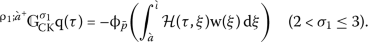
For $\mathrm{w}(\tau ) \in C^{+}(J)$, fractional boundary value problem (18) has a unique solution

$$\begin{aligned} \mathrm{q}(\tau ) & = \int _{\grave{a}}^{\grave{\iota}} \mathcal{G}_{1}( \tau , \xi ) \upphi _{\bar{p}} \biggl( \int _{\grave{a}}^{ \grave{\iota}} \mathcal{H}(\xi , s) \mathrm{w}(s) \,{\mathrm {d}}s \biggr) \,{\mathrm {d}}\xi \\ &\quad {} + \mu \biggl( \frac{\tau ^{\uprho _{1}} - \grave{a}^{\uprho _{1}}}{ \uprho _{1} - \mu \uprho _{1}} \biggr) \int _{\grave{a}}^{\grave{\iota}} \mathcal{G}_{2}( \tau , \xi ) \upphi _{\bar{p}} \biggl( \int _{\grave{a}}^{\grave{\iota}} \mathcal{H}(\xi , s) \mathrm{w}(s) \,{\mathrm {d}}s \biggr) \,{\mathrm {d}}\xi \\ &\quad {} + \lambda \biggl( \frac{\tau ^{\uprho _{1}} - \grave{a}^{\uprho _{1}}}{\uprho _{1} - \mu \uprho _{1}} \biggr) + F_{\circ } \biggl( \upphi _{\bar{p}} \biggl( \int _{ \grave{a}}^{\grave{\iota}} \mathcal{H}(\grave{a}, \xi ) \mathrm{w} ( \xi ) \,{\mathrm {d}}\xi \biggr) \biggr), \end{aligned}$$

(19)

where

$$ \mathcal{H}(\tau , \xi ) = \textstyle\begin{cases} \frac{1}{\Gamma (\sigma _{2}-1)} ( \frac{\grave{\iota}^{\uprho _{2}} - \tau ^{\uprho _{2}} }{ \uprho _{2}} ) ( \frac{\xi ^{\uprho _{2}} - \grave{a}^{\uprho _{2}}}{\uprho _{2}} )^{\sigma _{2} - 2} \xi ^{\uprho _{2}-1} \\ \quad {} - \frac{1}{ \Gamma ( \sigma _{2})} ( \frac{\xi ^{\uprho _{2}} - \tau ^{\uprho _{2}}}{ \uprho _{2}} )^{ \sigma _{2} -1} \xi ^{\uprho _{2}-1},& \tau \leq \xi , \\ \frac{1}{\Gamma (\sigma _{2}-1)} ( \frac{\grave{\iota}^{\uprho _{2}} - \tau ^{\uprho _{2}}}{ \uprho _{2}} ) ( \frac{\xi ^{\uprho _{2}} - \grave{a}^{\uprho _{2}}}{ \uprho _{2}} )^{\sigma _{2}- 2} \xi ^{\uprho _{2}-1},& \xi \leq \tau ,\end{cases} $$

(20)

$\mathcal{G}_{1}(\tau , \xi )$, $\mathcal{G}_{2}(\tau , \xi )$ are defined in Lemma 3.1and $\bar{p} = \frac{p}{p-1}$.

Proof

From Lemma 2.6, equation (18) is equivalent to the equation

for some constants $l_0,l_1,l_2\in \mathbb{R}$. Using the second boundary condition, we get

Consequently,

Thus, problem (18) can be written as

(21)

which, according to Lemma 3.1, has a unique solution of the form (19). □

Lemma 3.3

The functions $\mathcal{G}_{1}$, $\mathcal{G}_{2}$, and $\mathcal{H}$, equations (16), (17), and (20) satisfy the following:

• (i) $\mathcal{G}_{1}(\tau , \xi )$, $\mathcal{G}_{2}(\tau , \xi )$, and $\mathcal{H}(\tau , \xi )$ are continuous on $[\grave{a}, \grave{\iota}] \times [\grave{a}, \grave{\iota}]$.

• (ii) For all $(\tau , \xi ) \in [\grave{a}, \grave{\iota}]\times [\grave{a}, \grave{\iota}]$,

  $$\begin{aligned}& \begin{aligned} \mathcal{G}_{1} (\tau , \xi ) & \leqslant \biggl( \frac{\grave{\iota}^{\uprho _{1}} - \grave{a}^{\uprho _{1}} }{ \uprho _{1}} \biggr)^{\sigma _{1} -1 } \frac{ \grave{\iota}^{\uprho _{1} - 1 }}{ \Gamma (\sigma _{1} -1)} \int _{\grave{a}}^{\grave{\iota}} \mathcal{G}_{1}( \tau , \xi ) \,{\mathrm {d}}\xi \\ & = \biggl( \frac{\tau ^{\uprho _{1}} - \grave{a}^{\uprho _{1}}}{ \Gamma (\sigma _{1}) \uprho _{1}} \biggr) \biggl( \frac{ \grave{\iota}^{\uprho _{1}} - \grave{a}^{ \uprho _{1}}}{ \uprho _{1}} \biggr)^{ \sigma _{1} -1} \\ &\quad {} - \frac{1}{\Gamma (\sigma _{1} + 1 ) } \biggl( \frac{\tau ^{\uprho _{1}} - \grave{a}^{ \uprho _{1}}}{ \uprho _{1}} \biggr)^{\sigma _{1}}, \end{aligned} \\& \begin{aligned} \mathcal{G}_{2}(\tau , \xi ) & \leqslant \biggl( \frac{\grave{\iota }^{\uprho _{1}} - \grave{a}^{\uprho _{1}} }{ \uprho _{1}} \biggr)^{\sigma _{1} -2 } \frac{\grave{\iota}^{ \uprho _{1}- 1} }{ \Gamma (\sigma _{1} -1)} \int _{\grave{a}}^{\grave{\iota}} \mathcal{G}_{2}( \tau , \xi ) \,{\mathrm {d}}\xi \\ & = \frac{1}{ \Gamma (\sigma _{1})} \biggl( \biggl( \frac{\grave{ \iota}^{\uprho _{1}} - \grave{a}^{\uprho _{1}}}{ \uprho _{1}} \biggr)^{\sigma _{1} -1} - \biggl( \frac{ \tau ^{ \uprho _{1}} - \grave{a}^{\uprho _{1}}}{ \uprho _{1}} \biggr)^{\sigma _{1} - 1} \biggr), \end{aligned} \\& \begin{aligned} \mathcal{H} (\tau , \xi ) & \leqslant \biggl( \frac{\grave{\iota}^{\uprho _{2}} - \grave{a}^{\uprho _{2}} }{ \uprho _{2}} \biggr)^{ \sigma _{2} -1 } \frac{ \grave{\iota}^{ \uprho _{2} - 1}}{ \Gamma (\sigma _{2} -1)} \int _{\grave{a}}^{\grave{\iota}} \mathcal{H}(\tau , \xi ) \,{\mathrm {d}}\xi \\ & = \frac{\grave{\iota}^{\uprho _{2}} - \xi ^{\uprho _{2}}}{\uprho _{2} \Gamma (\sigma _{2})} \biggl( \biggl( \frac{ \grave{\iota}^{\uprho _{2}} - \grave{a}^{\uprho _{2}} }{ \uprho _{2}} \biggr)^{\sigma _{2} -1} - \frac{1}{\sigma _{2}} \biggl( \frac{ \grave{\iota}^{\uprho _{2}} - \xi ^{\uprho _{2}}}{ \uprho _{2} } \biggr)^{\sigma _{2} -1} \biggr). \end{aligned} \end{aligned}$$

• (iii) For all $(\tau , \xi ) \in [\grave{a}, \grave{\iota}]^{2} : \mathcal{G}_{1}( \tau , \xi ) \geqslant 0$, $\mathcal{G}_{2}(\tau , \xi ) \geqslant 0$, $\mathcal{H}(\tau , \xi )\geqslant 0$.

• (iv) For all $\xi \in J$, the function $\tau \to \mathcal{G}_{1}(\tau , \xi )$ is increasing and $\tau \to \mathcal{H}(\tau , \xi )$ is decreasing. In addition, $\forall (\tau , \xi ) \in (\grave{a}, \grave{\iota})^{2}$ we have

  $$ \biggl( \frac{\tau ^{\uprho _{1}} - \grave{a}^{\uprho _{1}}}{ \grave{\iota}^{\uprho _{1}} - \grave{a}^{\uprho _{1}}} \biggr)^{\sigma _{1} -1} \mathcal{G}_{1}( \grave{\iota}, \xi ) \leqslant \mathcal{G}_{1}(\tau , \xi ) $$

  and

  $$ \biggl( \frac{\grave{\iota}^{\uprho _{2}} - \tau ^{ \uprho _{2}}}{ \grave{\iota}^{\uprho _{2}} - \grave{a}^{ \uprho _{2}}} \biggr)^{\sigma _{2}-1} \mathcal{H}(\grave{a}, \xi ) \leqslant \mathcal{H}(\tau , \xi ). $$

• (v) For all $(\tau , \xi ) \in (\grave{a}, \grave{\iota})^{2}$, we have

  $$\begin{aligned} &\frac{\tau ^{\uprho _{1}-1} \uprho _{1}}{ \grave{\iota}^{\uprho _{1}} - \grave{a}^{\uprho _{1}}} \biggl[ 1 - \biggl( \frac{\tau}{ \grave{\iota}} \biggr)^{\uprho _{1}( \sigma _{1} -2)} \biggr] \mathcal{G}_{1}(\grave{\iota}, \xi ) \\ &\quad \leqslant {\mathcal{G}_{1}^{\prime}}_{\tau }(\tau , \xi ) \leqslant \frac{\sigma _{1}-1}{\sigma _{1} -2 } \frac{\tau ^{\uprho _{1}-1} \uprho _{1}}{ \grave{\iota}^{\uprho _{1}} - \grave{a}^{\uprho _{1}}} \mathcal{G}_{1}( \grave{\iota}, \xi ). \end{aligned}$$

Proof

Using the definitions of $\mathcal{G}_{1}$, $\mathcal{G}_{2}$, and $\mathcal{H}$, (i) and (ii) are obtained straightforwardly. For property (iii), we only consider the case $\xi \leq \tau$ as the other case is straightforward. When $\xi \leq \tau$, we have

$$\begin{aligned} \mathcal{G}_{1}(\tau , \xi ) & \geqslant \frac{1}{ \Gamma (\sigma _{1} -1) } \biggl( \frac{\tau ^{\uprho _{1}} - \xi ^{\uprho _{1}}}{ \uprho _{1}} \biggr) \biggl( \frac{\tau ^{\uprho _{1}} - \xi ^{ \uprho _{1}}}{\uprho _{1}} \biggr)^{\sigma _{1} - 2 } \grave{a}^{\uprho _{1}-1} \\ &\quad {} - \frac{1}{ \Gamma ( \sigma _{1})} \biggl( \frac{\tau ^{\uprho _{1}} - \xi ^{\uprho _{1}}}{ \uprho _{1}} \biggr)^{ \sigma _{1} -1} \grave{a}^{\uprho _{1} -1} \\ &\geqslant \biggl( \frac{ \tau ^{ \uprho _{1}} - \xi ^{\uprho _{1}}}{ \uprho _{1}} \biggr)^{\sigma _{1} -1} \grave{a}^{\uprho _{1} - 1 } \biggl[ \frac{1}{ \Gamma (\sigma _{1} -1)} - \frac{1}{ \Gamma (\sigma _{1})} \biggr]\geqslant 0, \end{aligned}$$

because $\Gamma (\sigma _{1} -1) \leqslant \Gamma (\sigma _{1})$ for $2 < \sigma _{1}\leq 3$. Similarly, we can easily prove that $\mathcal{G}_{2}(\tau , \xi )\geqslant 0$ and $\mathcal{H}(\tau , \xi )\geqslant 0$, $\forall (\tau , \xi ) \in J^{2}$. Now, for property (iv), we first check that $\mathcal{G}_{1}(\tau , \xi )$ is nondecreasing w.r.t. $\tau \in J$.

$$ \frac{\partial \mathcal{G}_{1}}{\partial \tau} (\tau , \xi )= \textstyle\begin{cases} \frac{\tau ^{\uprho _{1}-1}}{\Gamma (\sigma _{1} - 1) } ( \frac{\grave{\iota}^{\uprho _{1}} - \xi ^{\uprho _{1}}}{ \uprho _{1}} )^{ \sigma _{1} - 2 } \xi ^{\uprho _{1}-1} & \\ \quad {} - \frac{ \tau ^{\uprho _{1} - 1}}{ \Gamma ( \sigma _{1} -1) } ( \frac{\tau ^{ \uprho _{1}} - \xi ^{\uprho _{1}} }{ \uprho _{1}} )^{\sigma _{1} - 2 } \xi ^{\uprho _{1} -1},& \xi \leqslant \tau , \\ \frac{\tau ^{\uprho _{1} - 1}}{ \Gamma (\sigma _{1} -1 )} ( \frac{ \grave{\iota}^{\uprho _{1}} - \xi ^{\uprho _{1}}}{ \uprho _{1}} )^{\sigma _{1} - 2} \xi ^{\uprho _{1}-1},& \tau \leqslant \xi .\end{cases} $$

(22)

Thus, $\mathcal{G}_{1}(\tau , \xi )$ is increasing with respect to $\tau \in J$, and therefore $\mathcal{G}_{1}(\tau , \xi ) \leqslant \mathcal{G}_{1}(\grave{\iota}, \xi )$ for $\grave{a} \leqslant \tau$, $\xi \leqslant \grave{\iota}$. Furthermore, for $\tau \leqslant \xi$, we have

$$\begin{aligned} \frac{\partial \mathcal{H}(\tau , \xi ) }{\partial \tau} &= - \frac{\tau ^{\uprho _{2} - 1}}{ \Gamma (\sigma _{2} -1)} \biggl( \frac{\xi ^{\uprho _{2}} - \grave{a}^{\uprho _{2}}}{ \uprho _{2}} \biggr)^{\sigma _{2} - 2} \xi ^{\uprho _{2}-1} \\ &\quad {} + \frac{ ( \sigma _{2} -1 ) \tau ^{ \uprho _{2}-1}}{ \Gamma (\sigma _{2})} \biggl( \frac{ \xi ^{\uprho _{2}} - \tau ^{ \uprho _{2}}}{ \uprho _{2}} \biggr)^{\sigma _{2} -2} \xi ^{\uprho _{2}-1} \\ & = \frac{ \tau ^{\uprho _{2}-1}}{ \Gamma (\sigma _{2} - 1)} \xi ^{ \uprho _{2} -1} \biggl[ \biggl( \frac{\xi ^{\uprho _{2}} - \tau ^{\uprho _{2}}}{ \uprho _{2} } \biggr)^{\sigma _{2} -2} - \biggl( \frac{ \xi ^{\uprho _{2}} - \grave{a}^{\uprho _{2}}}{ \uprho _{2}} \biggr)^{\sigma _{2} -2} \biggr] \\ &\leqslant \frac{ \tau ^{ \uprho _{2}-1}}{ \Gamma (\sigma _{2}-1)} \xi ^{\uprho _{2} -1} \biggl[ \biggl( \frac{ \xi ^{\uprho _{2}} - \grave{a}^{\uprho _{2}}}{\uprho _{2}} \biggr)^{\sigma _{2} -2} - \biggl( \frac{\xi ^{\uprho _{2}} - \grave{a}^{\uprho _{2}}}{ \uprho _{2}} \biggr)^{\sigma _{2} -2} \biggr]= 0, \end{aligned}$$

and for $\xi \leqslant \tau$, we have

$$\begin{aligned} \frac{ \mathcal{H}(\tau , \xi ) }{\partial \tau} &= \frac{ - \tau ^{ \uprho _{2}-1}}{ \Gamma (\sigma _{2} - 1)} \biggl( \frac{\xi ^{\uprho _{2}} - \grave{a}^{\uprho _{2}}}{ \uprho _{2}} \biggr)^{\sigma _{2} -2} \xi ^{\uprho _{2}-1} \leqslant 0. \end{aligned}$$

Thus, $\mathcal{H}(\tau , \xi )$ is nonincreasing with respect to τ. Consequently, $\mathcal{H}(\tau , \xi )\leqslant \mathcal{H}(\grave{a}, \xi )$, $\forall \tau , \xi \in J$. On the other hand, when $\tau \geqslant \xi$,

$$\begin{aligned} \frac{\mathcal{G}_{1}(\tau , \xi )}{\mathcal{G}_{1}(\grave{\iota}, \xi )} & = \frac{ (\sigma _{1} - 1) ( \tau ^{\uprho _{1}} - \grave{a}^{\uprho _{1}}) (\grave{\iota}^{\uprho _{1}} - \xi ^{\uprho _{1}})^{\sigma _{1}-2} - (\tau ^{\uprho _{1}} - \xi ^{\uprho _{1}})^{ \sigma _{1} -1} }{ (\sigma _{1} -1) (\grave{\iota}^{\uprho _{1}} - \grave{a}^{\uprho _{1}}) (\grave{\iota}^{\uprho _{1}} - \xi ^{\uprho _{1}})^{\sigma _{1}-2} - (\grave{\iota}^{\uprho _{1} } - \xi ^{\uprho _{1}})^{\sigma _{1} -1} } \\ & = \frac{1}{ (\sigma _{1} -1) (\grave{\iota}^{\uprho _{1}} - \grave{a}^{\uprho _{1}}) ( \grave{\iota}^{\uprho _{1}} - \xi ^{\uprho _{1}})^{\sigma _{1}-2} - ( \grave{\iota}^{ \uprho _{1}} - \xi ^{\uprho _{1}})^{\sigma _{1} -1} } \\ &\quad {} \times \biggl[ (\sigma _{1}-1) \bigl(\tau ^{\uprho _{1}} - \grave{a}^{ \uprho _{1}}\bigr) \bigl(\grave{\iota}^{\uprho _{1}} - \xi ^{\uprho _{1}}\bigr)^{ \alpha -2} \\ &\quad {} - \bigl(\tau ^{ \uprho _{1}} - \xi ^{\uprho _{1}}\bigr)^{\sigma _{1} -1} \biggl( \frac{\tau ^{\uprho _{1}} - \xi ^{\uprho _{1}} }{ \tau ^{\uprho _{1}} - \grave{a}^{\uprho _{1}}} \biggr)^{\sigma _{1} -1} \biggr]. \end{aligned}$$

As

$$ \biggl( \frac{\tau ^{\uprho} - \xi ^{\uprho}}{ \tau ^{\uprho} - \grave{a}^{\uprho}} \biggr)^{\sigma} \leq \biggl( \frac{\grave{\iota}^{\uprho} - \xi ^{\uprho}}{ \grave{ \iota}^{ \uprho} - \grave{a}^{\uprho}} \biggr)^{\sigma},$$

for $\sigma >0$, we obtain

$$\begin{aligned} \frac{ \mathcal{G}_{1}( \tau , \xi )}{\mathcal{G}_{1} ( \grave{\iota}, \xi )} & \geqslant \frac{1}{ (\sigma _{1} -1) (\grave{\iota}^{\uprho _{1}} - \grave{a}^{\uprho _{1}}) ( \grave{\iota}^{\uprho _{1}} - \xi ^{\uprho _{1}})^{\sigma _{1}-2} - ( \grave{\iota}^{ \uprho _{1}} - \xi ^{\uprho _{1}})^{\sigma _{1} -1} } \\ &\quad {} \times \biggl[ (\sigma _{1}-1) \bigl(\tau ^{\uprho _{1}} - \grave{a}^{\uprho _{1}}\bigr) \bigl( \grave{\iota}^{\uprho _{1} } - \xi ^{ \uprho _{1}}\bigr)^{\sigma _{1}-2} \\ &\quad {} - \bigl(\tau ^{ \uprho _{1}} - \xi ^{\uprho _{1}}\bigr)^{\sigma _{1} -1} \biggl( \frac{\grave{ \iota}^{\uprho _{1}} - \xi ^{\uprho _{1}} }{ \grave{\iota}^{ \uprho _{1}} - \grave{a}^{\uprho _{1}}} \biggr)^{\sigma _{1} -1} \biggr] \\ & \geqslant \frac{ ( \tau ^{ \uprho _{1}} - \grave{a}^{\uprho _{1}})^{\sigma _{1} - 1 } }{ (\grave{\iota}^{ \uprho _{1}} - \grave{a}^{\uprho _{1}} )^{\sigma _{1}-1} } \\ &\quad {} \times \frac{1}{ (\sigma _{1}-1 ) ( \grave{\iota}^{ \uprho _{1}} - \grave{a}^{ \uprho _{1}}) ( \grave{\iota}^{ \uprho _{1}} - \xi ^{\uprho _{1}} )^{\sigma _{1} -2} - ( \grave{ \iota}^{ \uprho _{1}} - \xi ^{ \uprho _{1}} )^{\sigma _{1} -1} } \\ &\quad {}\times \bigl[ (\sigma _{1} -1) \bigl( \grave{\iota}^{\uprho _{1}} - \grave{a}^{\uprho _{1}} \bigr)^{\sigma _{1} -1} \bigl(\tau ^{\uprho _{1}} - \grave{a}^{ \uprho _{1}}\bigr)^{2 - \sigma _{1}} \bigl( \grave{ \iota}^{ \uprho _{1}} - \xi ^{ \uprho _{1}}\bigr)^{\sigma _{1} - 2} \\ &\quad {} - \bigl( \grave{\iota}^{ \uprho _{1} } -\xi ^{ \uprho _{1} } \bigr)^{ \sigma _{1} -1} \bigr] \\ & \geqslant \frac{ (\tau ^{ \uprho _{1} } - \grave{a}^{\uprho _{1}})^{\sigma _{1} -1 }}{ ( \grave{\iota}^{ \uprho _{1}} - \grave{a}^{\uprho _{1}} )^{\sigma _{1} -1} } \\ &\quad {} \times \frac{1}{ (\sigma _{1} - 1) ( \grave{\iota}^{\uprho _{1}} - \grave{a}^{\uprho _{1}}) ( \grave{\iota}^{ \uprho _{1}} - \xi ^{ \uprho _{1}})^{ \sigma _{1} -2} - ( \grave{\iota}^{ \uprho _{1}} - \xi ^{\uprho _{1}})^{\sigma _{1} -1} } \\ &\quad {} \times \biggl[ \biggl( \frac{ \grave{ \iota}^{ \uprho _{1}} - \grave{a}^{ \uprho _{1} } }{ \tau ^{ \uprho _{1} } - \grave{a}^{ \uprho _{1}}} \biggr)^{ \sigma _{1} -2} (\sigma _{1} -1) \bigl( \grave{\iota}^{ \uprho _{1}} - \grave{a}^{ \uprho _{1}} \bigr) \bigl( \grave{\iota}^{ \uprho _{1}} - \xi ^{ \uprho _{1}}\bigr)^{\sigma _{1} -2} \\ &\quad {} - \bigl( \grave{\iota}^{ \uprho _{1}} - \xi ^{ \uprho _{1}} \bigr)^{\sigma _{1} -1} \biggr] \\ & \geqslant \frac{ (\tau ^{ \uprho _{1}} - \grave{a}^{\uprho _{1}} )^{ \sigma _{1} - 1 } }{ ( \grave{\iota}^{\uprho _{1}} - \grave{a}^{ \uprho _{1} } )^{\sigma _{1} -1} }. \end{aligned}$$

For $\tau \leqslant \xi$, we have

$$ \frac{ \mathcal{G}_{1}(\tau , \xi )}{ ( \tau ^{ \uprho _{1}} - \grave{a}^{\uprho _{1}} )^{\sigma _{1} -1}} = \frac{ \uprho _{1}^{\sigma _{1} -1} \xi ^{\uprho _{1} - 1}}{ \Gamma (\sigma _{1} - 1)} \bigl( \grave{ \iota}^{ \uprho _{1}} - \xi ^{ \uprho _{1}} \bigr)^{ \sigma _{1} -2} \frac{1}{ (t^{\uprho _{1}} - \grave{a}^{\uprho _{1} } )^{ \sigma _{1} -2}},$$

which is a nonincreasing function as $\sigma _{1} \geq 0$. Consequently,

$$ \frac{\mathcal{G}_{1}(\tau , \xi )}{ ( \tau ^{\uprho _{1}} - \grave{a}^{\uprho _{1}} )^{\sigma _{1} -1}} \geq \frac{ \mathcal{G} (\grave{\iota}, \xi )}{ ( \grave{\iota}^{\uprho _{1}} - \grave{a}^{\uprho _{1}} )^{\sigma _{1} - 1}},$$

which implies

$$ \mathcal{G}_{1}( \tau , \xi ) \geqslant \biggl( \frac{ \tau ^{ \uprho _{1} } - \grave{a}^{\uprho _{1}} }{ \grave{\iota}^{ \uprho _{1}} - \grave{a}^{\uprho _{1}} } \biggr)^{\sigma _{1} -1} \mathcal{G}_{1} ( \grave{\iota}, \xi ).$$

Using similar techniques, one can prove that

$$ \mathcal{H}(\tau , \xi ) \geqslant \biggl( \frac{ \grave{\iota}^{\uprho _{2}} - \tau ^{ \uprho _{2}} }{ \grave{\iota}^{ \uprho _{2}} - \grave{a}^{ \uprho _{2}}} \biggr)^{ \sigma -1} \mathcal{H}(\grave{a}, \xi )$$

for $\grave{a} \leqslant \xi , \tau < \grave{\iota}$. Therefore (iv) of Lemma 3.3 holds. Finally, for property (v), we can consider two cases. Nevertheless, we prove the results for the case $\xi \leq \tau$ only. The simpler case $\grave{a} \leq \tau \leq \xi < \grave{ \iota}$ can be treated with similar arguments. When $\xi \leq \tau$, we have

$$ \frac{{\mathcal{G}_{1}}_{\tau}^{\prime}(\tau , \xi )}{ \mathcal{G}_{1}( \grave{\iota}, \xi ) } \frac{ ( \grave{\iota}^{\uprho _{1}} - \grave{a}^{ \uprho _{1}}) }{\tau ^{\uprho _{1} - 1} \uprho _{1} (\sigma _{1} - 1 ) } = \frac{ ( \grave{\iota}^{ \uprho _{1}} - \xi ^{ \uprho _{1} } )^{ \sigma _{1} - 2 } - ( \tau ^{ \uprho _{1}} - \xi ^{ \uprho _{1} } )^{\sigma _{1} -2}}{(\sigma _{1} - 1) ( \grave{\iota}^{\uprho _{1}} - \xi ^{ \uprho _{1} } )^{\sigma _{1} -2} - \frac{ ( \grave{\iota}^{ \uprho _{1}} - \xi ^{ \uprho _{1}} )^{\sigma _{1} -1} }{ ( \grave{\iota}^{\uprho _{1}} - \grave{a}^{\uprho _{1}})}}. $$

Consequently,

$$\begin{aligned} \frac{{\mathcal{G}_{1}}_{\tau}^{\prime}(\tau , \xi )}{\mathcal{G}_{1}(\grave{\iota}, \xi )} \frac{(\grave{\iota}^{\uprho _{1}} - \grave{a}^{\uprho _{1}}) }{ \tau ^{\uprho _{1} - 1} \uprho _{1} (\sigma _{1} -1)} & \leq \frac{ ( \grave{ \iota}^{ \uprho _{1}} - \xi ^{ \uprho _{1}} )^{\sigma _{1} -2} }{ (\sigma _{1} -1) ( \grave{\iota}^{ \uprho _{1}} - \xi ^{\uprho _{1}} )^{\sigma _{1} -2} - \frac{ ( \grave{\iota}^{ \uprho _{1}} - \xi ^{\uprho _{1}} )^{ \sigma _{1} -1}}{ (\grave{\iota}^{\uprho _{1}} - \grave{a}^{\uprho _{1}})}} \\ & \leq \frac{1}{(\sigma _{1}-1) - \frac{ (\grave{\iota}^{ \uprho _{1}} - \xi ^{ \uprho _{1}} )}{ ( \grave{\iota}^{ \uprho _{1}} - \grave{a}^{\uprho _{1}})}} \\ & \leq \frac{1}{(\sigma _{1} - 2)}. \end{aligned}$$

On the other hand,

$$\begin{aligned} \frac{{\mathcal{G}_{1}}_{\tau}^{\prime}(\tau , \xi )}{ \mathcal{G}_{1}( \grave{\iota}, \xi )} \frac{(\grave{\iota}^{\uprho _{1}} - \grave{a}^{\uprho _{1}}) }{\tau ^{\uprho _{1}-1} \uprho _{1} } & = \frac{(\sigma _{1} -1) [ ( \grave{\iota}^{ \uprho _{1}} - \xi ^{ \uprho _{1}} )^{ \sigma _{1} -2} - ( \tau ^{ \uprho _{1}} - \xi ^{\uprho _{1} } )^{\sigma _{1} -2} ]}{(\sigma _{1}-1) ( \grave{\iota}^{ \uprho _{1}} - \xi ^{\uprho _{1}} )^{\sigma _{1} -2} - \frac{ ( \grave{\iota}^{ \uprho _{1}} - \xi ^{\uprho _{1}} )^{ \sigma _{1} -1}}{( \grave{\iota}^{\uprho _{1}} - \grave{a}^{ \uprho _{1}})}} \\ & \geq 1 - \frac{ ( \tau ^{ \uprho _{1}} - \xi ^{\uprho _{1}} )^{ \sigma _{1} -2}}{ ( \grave{ \iota}^{ \uprho _{1}} - \xi ^{\uprho _{1}} )^{ \sigma _{1} -2} } \\ & \geq 1 - \biggl( \frac{\tau}{ \grave{\iota}} \biggr)^{ \uprho _{1} ( \sigma _{1} -2)} \biggl( \frac{ 1 - ( \frac{\xi}{\tau} )^{ \uprho _{1}}}{ 1 - ( \frac{\xi}{ \grave{\iota}} )^{ \uprho _{1}}} \biggr)^{\sigma _{1} -2} \\ & \geq 1 - \biggl( \frac{\tau}{\grave{\iota}} \biggr)^{ \uprho _{1} ( \sigma _{1} -2)}. \end{aligned}$$

Thus, the proof is completed. □

Now, consider the Banach space $\mathbb{E}=C_{{\mathrm{\rho }}_1}^3(J)$. Suppose that is continuous on J for all $\mathrm{q}\in \mathbb{E}$, then from Definition 2.6 and Lemma 2.4 we can define the norm on $\mathbb{E}$ as follows:

in which

$$ \breve{M}_{1}=\max \Bigl\{ \max_{\tau \in J} \bigl\vert \mathrm{q}(\tau ) \bigr\vert , \max_{\tau \in J} \bigl\vert \delta _{\uprho _{1}}^{1} \mathrm{q}(\tau ) \bigr\vert , \max_{\tau \in J} \bigl\vert \delta _{ \uprho _{1}}^{2} \mathrm{q}(\tau ) \bigr\vert \Bigr\} ,$$

and the cone

$$K=\{\mathrm{q}\in \mathbb{E}:\mathrm{q}\text{ is nonnegative, increasing, and }{\mathrm{\rho }}_1\text{-concave}\}.$$

Lemma 3.4

Assume (H2) and let q be the unique solution of fractional boundary value problem (18) associated with given $\mathrm{w}(\tau )\in C^{+}(J)$. Then $\mathrm{q}\in K$ and the following inequalities hold for $\tau \in [\grave{a}_{\circ}, \grave{\iota}_{\circ}] \subset ( \grave{a}, \grave{\iota})$:

$$\begin{aligned}& \max_{\tau \in J} \bigl\vert \mathrm{q}(\tau ) \bigr\vert \leqslant \biggl( \biggl( \frac{ \grave{a}_{\circ}^{ \uprho _{1}} - \grave{a}^{ \uprho _{1}}}{ \grave{\iota}^{ \uprho _{1}} - \grave{a}^{\uprho _{1}}} \biggr)^{\sigma _{1} -1 } \biggl( \frac{ \grave{ \iota}^{\uprho _{2}}- \grave{\iota}_{\circ}^{\uprho _{2}}}{\grave{\iota}^{\uprho _{2}} - \grave{a}^{ \uprho _{2}}} \biggr)^{ \sigma _{1} - 1} \biggr)^{-1} \mathrm{q}(\tau ), \end{aligned}$$

(23)

$$\begin{aligned}& \max_{\tau \in J} \bigl\vert \delta _{\uprho _{1}}^{1} \mathrm{q}(\tau ) \bigr\vert \leqslant \frac{\sigma _{1} -1}{ \sigma _{1} - 2 } \frac{\uprho _{1}}{ \grave{\iota}^{ \uprho _{1}} - \grave{a}^{\uprho _{1}}} \max_{ \tau \in J} \bigl\vert \mathrm{q}(\tau ) \bigr\vert , \end{aligned}$$

(24)

$$\begin{aligned}& \begin{aligned}[b] \max_{\tau \in J} \bigl\vert \delta _{\uprho _{1}}^{2} \mathrm{q}(\tau ) \bigr\vert & \leqslant \biggl( \biggl( \frac{ \grave{a}_{\circ}^{\uprho _{1}} - \grave{a}^{\uprho _{1}}}{ \grave{\iota}^{ \uprho _{1}}- \grave{a}^{ \uprho _{1}}} \biggr)^{ \sigma _{1}-1} Z(\grave{ \iota}_{\circ}) \int ^{ \grave{ \iota}}_{ \grave{a}} \mathcal{G}_{1}( \grave{\iota}, \xi ) \,{\mathrm {d}}\xi \biggr)^{-1} \\ & \quad {}\times \frac{1}{ \Gamma (\sigma _{1} - 1) } \biggl( \frac{ \grave{\iota}^{\uprho _{1}} - \grave{a}^{\uprho _{1}}}{\uprho _{1}} \biggr)^{ \sigma _{1} -2} \max_{\tau \in J} \bigl\vert \mathrm{q}( \tau ) \bigr\vert , \end{aligned} \end{aligned}$$

(25)

(26)

$$\begin{aligned}& \min_{\tau \in [\grave{a}_{\circ}, \grave{\iota}_{\circ}] } \mathrm{q}(\tau ) \geqslant \biggl( \frac{ \grave{a}_{\circ}^{\uprho _{1}} - \grave{a}^{\uprho _{1}}}{ \grave{\iota}^{ \uprho _{1}} - \grave{a}^{ \uprho _{1}}} \biggr)^{\sigma _{1}-1} \breve{M}_{2} \Vert \mathrm{q} \Vert , \end{aligned}$$

(27)

where

$$ Z(\tau ) = \upphi _{\bar{p}} \biggl( \biggl( \frac{ \grave{\iota}^{\uprho _{2}} - \tau ^{ \uprho _{2}}}{ \grave{\iota}^{ \uprho _{2}} - \grave{a}^{\uprho _{2}}} \biggr)^{ \sigma _{2}-1} \biggr)$$

and

$$\begin{aligned} \breve{M}_{2} & = \min \biggl\lbrace 1, \frac{ \sigma _{1} -2}{\sigma _{1} -1} \biggl( \frac{ \grave{\iota}^{\uprho _{1}} - \grave{a}^{\uprho _{1}}}{ \uprho _{1}} \biggr), \\ &\quad \min \biggl\lbrace \Gamma (\sigma _{1} -1) \biggl( \frac{\grave{\iota}^{\uprho _{1}} - \grave{a}^{\uprho _{1}}}{ \uprho _{1}} \biggr)^{ 2 - \sigma _{1}}, 1 \biggr\rbrace \\ &\quad {} \times \biggl( \frac{ \grave{a}_{\circ}^{\uprho _{1}} - \grave{a}^{\uprho _{1}}}{ \grave{\iota}^{\uprho _{1}} - \grave{a}^{ \uprho _{1}}} \biggr)^{ \sigma _{1} -1} \times Z( \grave{\iota}_{\circ}) \int ^{ \grave{ \iota}}_{\grave{a}} \mathcal{G}_{1} ( \grave{\iota}, \xi ) \,{\mathrm {d}}\xi \biggr\rbrace . \end{aligned}$$

(28)

Proof

From Lemma 3.2, we have

$$\begin{aligned} \mathrm{q}(\tau ) & = \int _{\grave{a}}^{ \grave{\iota}} \mathcal{G}_{1}( \tau , \xi ) \upphi _{\bar{p}} \biggl( \int _{ \grave{a}}^{ \grave{\iota}} \mathcal{H}(\xi , s) \mathrm{w}(s) \,\mathrm{d} s \biggr) \,{\mathrm {d}}\xi \\ &\quad {} + \mu \biggl( \frac{\tau ^{\uprho _{1}} - \grave{a}^{\uprho _{1}}}{ \uprho _{1} - \mu \uprho _{1}} \biggr) \int _{\grave{a}}^{\grave{\iota}} \mathcal{G}_{2}( \tau , \xi ) \upphi _{\bar{p}} \biggl( \int _{\grave{a}}^{\grave{\iota}} \mathcal{H}(\xi , s) \mathrm{w}(s) \,\mathrm{d}s \biggr) \,{\mathrm {d}}\xi \\ &\quad {} + \lambda \biggl( \frac{\tau ^{\uprho _{1}} - \grave{a}^{\uprho _{1}}}{\uprho _{1} - \mu \uprho _{1}} \biggr) + F_{\circ } \biggl( \upphi _{\bar{p}} \biggl( \int _{ \grave{a}}^{\grave{\iota}} \mathcal{H}(\grave{a}, \xi ) \mathrm{w}( \xi ) \,\mathrm{d}\xi \biggr) \biggr). \end{aligned}$$

• (1) The functions $\mathcal{G}_{1}$, $\mathcal{G}_{2}$, and $\mathcal{H}$ are nonnegative (Lemma 3.3(iii)). In addition, $F_{\circ}(v)$ is nonnegative for $v\geq 0$ (thanks to (H2)). Thus, q is also nonnegative. Furthermore, as $\mathcal{G}_{1}$ is increasing w.r.t. τ (Lemma 3.3(iv)), so it is the function q. To prove that q is $\uprho _{1}$-concave, we need to show that $\delta _{ \uprho _{1}}^{1} \mathrm{q}(\tau )$ is decreasing on J (Remark 2.2), which can be obtained from the negativity of the derivative

  $$\begin{aligned} \bigl( \delta _{\uprho _{1}}^{1} \mathrm{q}(\tau ) \bigr)^{\prime} & = - \frac{\tau ^{ \uprho _{1} -1}}{ \Gamma (\sigma _{1} -2 )} \int _{ \grave{a}}^{\tau} \biggl( \frac{ \tau ^{\uprho _{1}} - \xi ^{ \uprho _{1}}}{ \uprho _{1}} \biggr)^{ \sigma _{1} -3} \xi ^{ \uprho _{1}-1} \\ &\quad {} \times \upphi _{\bar{p}} \biggl( \int _{\grave{a}}^{ \grave{\iota}} \mathcal{H}(\xi , s) \mathrm{w}(s) \,\mathrm{d} s \biggr) \,\mathrm{d} \xi \leq 0. \end{aligned}$$

• (2) As q is nonnegative and increasing, we have

  $$\begin{aligned} \max_{\tau \in J } \bigl\vert \mathrm{q}(\tau ) \bigr\vert & = \mathrm{q}(\grave{\iota}) \\ & = \int _{\grave{a}}^{\grave{\iota}} \mathcal{G}_{1}( \grave{\iota}, \xi ) \upphi _{\bar{p}} \biggl( \int _{\grave{a}}^{\grave{\iota}} \mathcal{H}(\xi , s) \mathrm{w}(s) \,\mathrm{d}s \biggr) \,\mathrm{d}\xi \\ &\quad {} + \mu \biggl( \frac{ \grave{\iota}^{\uprho _{1}} - \grave{a}^{\uprho _{1}}}{ \uprho _{1} - \mu \uprho _{1}} \biggr) \int _{\grave{a}}^{ \grave{\iota}} \mathcal{G}_{2}( \tau , \xi ) \upphi _{\bar{p}} \biggl( \int _{ \grave{a}}^{\grave{\iota}} \mathcal{H}(\xi , s) \mathrm{w}(s) \,\mathrm{d}s \biggr) \,\mathrm{d} \xi \\ &\quad {} + \lambda \biggl( \frac{\grave{ \iota}^{ \uprho _{1}} - \grave{a}^{ \uprho _{1}}}{ \uprho _{1} - \mu \uprho _{1}} \biggr) + F_{\circ} \biggl( \upphi _{\bar{p}} \biggl( \int _{\grave{a}}^{ \grave{\iota}} \mathcal{H}(\grave{a}, \xi ) \mathrm{w}(\xi ) \,\mathrm{d}\xi \biggr) \biggr). \end{aligned}$$

  For $\tau \in [\grave{a}_{\circ},\grave{\iota}_{\circ}]$, using (iv) of Lemma 3.3 and the fact that

  $$ \biggl( \frac{ \grave{a}_{\circ}^{\uprho _{1}}- \grave{a}^{\uprho _{1}}}{ \grave{\iota}^{ \uprho _{1}}- \grave{a}^{\uprho _{1}}} \biggr) < 1,$$

  we get

  $$\begin{aligned} \mathrm{q}(\tau )& \geqslant \int _{\grave{a}}^{\grave{\iota}} \biggl( \frac{\grave{a}_{\circ}^{\uprho _{1}} - \grave{a}^{ \uprho _{1}}}{ \grave{\iota}^{ \uprho _{1}}- \grave{a}^{\uprho _{1}}} \biggr)^{\sigma _{1} -1} \mathcal{G}_{1}(\grave{\iota}, \xi ) \upphi _{\bar{p}} \biggl( \int _{\grave{a}}^{\grave{\iota}} \mathcal{H}(\xi , s) \mathrm{w}(s) \,\mathrm{d}s \biggr) \,{\mathrm {d}}\xi \\ &\quad {} +\mu \biggl( \frac{ \grave{a}_{\circ}^{\uprho _{1}}- \grave{a}^{\uprho _{1}}}{\grave{\iota}^{\uprho _{1}}- \grave{a}^{ \uprho _{1}}} \biggr)^{\sigma _{1} -2} \biggl( \frac{\tau ^{\uprho _{1}} - \grave{a}^{\uprho _{1}}}{ \uprho _{1} - \mu \uprho _{1}} \biggr) \\ &\quad {} \times \int _{\grave{a}}^{\grave{\iota}} \mathcal{G}_{2}( \tau , \xi ) \upphi _{\bar{p}} \biggl( \int _{\grave{a}}^{ \grave{\iota}} \mathcal{H}(\xi , s) \mathrm{w}(s) \,\mathrm{d}s \biggr) \,{\mathrm {d}}\xi \\ &\quad {} +\lambda \biggl( \frac{\grave{a}_{\circ}^{\uprho _{1}}- \grave{a}^{\uprho _{1}}}{\grave{\iota}^{\uprho _{1}}- \grave{a}^{\uprho _{1}}} \biggr)^{\sigma _{1}-2} \biggl( \frac{\tau ^{\uprho _{1}}-\grave{a}^{\uprho _{1}}}{\uprho _{1} - \mu \uprho _{1}} \biggr) \\ &\quad {} + \biggl( \frac{\grave{a}_{\circ}^{ \uprho _{1}}- \grave{a}^{\uprho _{1}}}{ \grave{\iota}^{\uprho _{1}} - \grave{a}^{ \uprho _{1}}} \biggr)^{\sigma _{1}-1} F_{\circ} \biggl( \upphi _{\bar{p}} \biggl( \int _{\grave{a}}^{\grave{\iota}} \mathcal{H}( \grave{a}, \xi ) \mathrm{w}(\xi ) \,\mathrm{d}\xi \biggr) \biggr). \end{aligned}$$

  Consequently,

  $$ \mathrm{q}(\tau ) \geqslant \biggl( \frac{\grave{a}_{\circ}^{\uprho _{1}}- \grave{a}^{\uprho _{1}}}{\grave{\iota}^{\uprho _{1}}- \grave{a}^{\uprho _{1}}} \biggr)^{\sigma _{1} -1}\max_{t \in J} \bigl\vert \mathrm{q}( \tau ) \bigr\vert , $$

  and thus (23) holds.

• (3) We have

  $$\begin{aligned} \delta _{\uprho _{1}}^{1} \mathrm{q}(\tau ) & = \tau ^{1 - \uprho _{1}} \int _{\grave{a}}^{\grave{\iota}} {\mathcal{G}_{1}}^{\prime}_{\tau}( \tau , \xi ) \upphi _{\bar{p}} \biggl( \int _{\grave{a}}^{ \grave{\iota}} \mathcal{H}(\xi , s) \mathrm{w}(s) \,\mathrm{d}s \biggr) \,{\mathrm {d}}\xi \\ &\quad {} + \frac{\mu }{ (1-\mu )} \int _{ \grave{a}}^{ \grave{\iota}} \mathcal{G}_{2}( \tau , \xi ) \upphi _{\bar{p}} \biggl( \int _{\grave{a}}^{\grave{\iota}} \mathcal{H}(\xi , s) \mathrm{w}(s) \,\mathrm{d}s \biggr) \,{\mathrm {d}}\xi + \frac{\lambda }{(1-\mu )}. \end{aligned}$$

  From Lemma 3.3 ((iii) and (v)), we can deduce that $\delta _{\uprho _{1}}^{1} \mathrm{q}(\tau ) \geq 0$ and

  $$\begin{aligned} \delta _{\uprho _{1}}^{1} \mathrm{q}(\tau ) & \leqslant \int _{ \grave{a}}^{\grave{\iota}} \frac{ \sigma _{1}-1}{\sigma _{1} - 2} \frac{ \uprho _{1}}{ \grave{\iota}^{ \uprho _{1}} - \grave{a}^{\uprho _{1}}} \mathcal{G}_{1}( \grave{\iota}, \xi )\upphi _{\bar{p}} \biggl( \int _{ \grave{a}}^{\grave{\iota}} \mathcal{H}( \xi , s) \mathrm{w}(s) \,\mathrm{d}s \biggr) \,{\mathrm {d}}\xi \\ &\quad {} + \frac{\mu }{ (1-\mu )} \int _{\grave{a}}^{ \grave{\iota}} \mathcal{G}_{2}( \tau , \xi ) \upphi _{\bar{p}} \biggl( \int _{\grave{a}}^{\grave{\iota}} \mathcal{H}(\xi , s) \mathrm{w}(s) \,\mathrm{d} s \biggr) \,{\mathrm {d}}\xi + \frac{\lambda }{(1-\mu )} \\ & \leqslant \frac{ \sigma _{1}-1}{\sigma _{1} - 2} \frac{ \uprho _{1}}{ \grave{\iota}^{ \uprho _{1}} - \grave{a}^{ \uprho _{1}}} \biggl[ \int _{\grave{a}}^{\grave{\iota}} \mathcal{G}_{1}( \grave{\iota}, \xi ) \upphi _{\bar{p}} \biggl( \int _{\grave{a}}^{ \grave{\iota}} \mathcal{H}(\xi , s) \mathrm{w}(s) \,\mathrm{d} s \biggr) \,{\mathrm {d}}\xi \\ &\quad {} + \mu \biggl( \frac{\grave{\iota}^{\uprho _{1}} - \grave{a}^{\uprho _{1}} }{ \uprho _{1}-\mu \uprho _{1} } \biggr) \int _{\grave{a}}^{\grave{\iota}} \mathcal{G}_{2}( \tau , \xi ) \upphi _{\bar{p}} \biggl( \int _{\grave{a}}^{\grave{\iota}} \mathcal{H}(\xi , s) \mathrm{w}(s) \mathrm{s} s \biggr) \,{\mathrm {d}}\xi \\ &\quad {} + \lambda \biggl( \frac{\grave{\iota}^{ \uprho _{1}} - \grave{a}^{\uprho _{1}} }{ \uprho _{1} - \mu \uprho _{1} } \biggr) \biggr] \\ & \leqslant \frac{\sigma _{1}-1}{\sigma _{1}- 2} \frac{\uprho _{1}}{ \grave{\iota}^{ \uprho _{1}}-\grave{a}^{\uprho _{1}}} \biggl[ \int _{\grave{a}}^{\grave{\iota}} \mathcal{G}_{1}( \grave{\iota}, \xi )\upphi _{\bar{p}} \biggl( \int _{\grave{a}}^{ \grave{\iota}} \mathcal{H}(\xi , s) \mathrm{w}(s) \,\mathrm{d}s \biggr) \,{\mathrm {d}}\xi \\ &\quad {} + \lambda \biggl( \frac{\grave{\iota}^{\uprho _{1}} - \grave{a}^{\uprho _{1}} }{ \uprho _{1}- \mu \uprho _{1} } \biggr) \\ &\quad {} + \mu \biggl( \frac{ \grave{\iota}^{ \uprho _{1}} - \grave{a}^{\uprho _{1}} }{ \uprho _{1} -\mu \uprho _{1} } \biggr) \int _{\grave{a}}^{\grave{\iota}} \mathcal{G}_{2}( \tau , \xi ) \upphi _{\bar{p}} \biggl( \int _{ \grave{a}}^{ \grave{\iota}} \mathcal{H}(\xi , s) \mathrm{w}(s) \,\mathrm{d}s \biggr) \,{\mathrm {d}} \xi \\ &\quad {} + F_{\circ } \biggl(\upphi _{\bar{p}} \biggl( \int _{\grave{a}}^{ \grave{\iota}} \mathcal{H}(\grave{a}, \xi ) \mathrm{w}(\xi ) \,\mathrm{d}\xi \biggr) \biggr) \biggr] \\ & \leqslant \frac{\sigma _{1}-1}{\sigma _{1} - 2} \frac{\uprho _{1}}{\grave{\iota}^{\uprho _{1}}-\grave{a}^{\uprho _{1}}} \mathrm{q}( \grave{\iota}). \end{aligned}$$

  Thus, we obtain (24).

• (4) A straightforward calculus gives

  $$\begin{aligned} \delta _{\uprho _{1}}^{2} \mathrm{q}(\tau ) & = - \frac{1}{\Gamma (\sigma _{1} -2) } \int _{\grave{a}}^{\tau} \biggl( \frac{\tau ^{\uprho _{1}} - \xi ^{\uprho _{1}}}{\uprho _{1}} \biggr)^{ \sigma _{1} -3} \xi ^{\uprho _{1}-1} \\ & \quad {}\times \upphi _{\bar{p}} \biggl( \int _{\grave{a}}^{ \grave{\iota}} \mathcal{H}(\xi , s) \mathrm{w}(s) \,{\mathrm {d}}s \biggr) \,{\mathrm {d}}\xi . \end{aligned}$$

  Then we get

  $$\begin{aligned} \bigl\vert \delta _{\uprho _{1}}^{2} \mathrm{q}(\tau ) \bigr\vert & \leqslant \upphi _{\bar{p}} \biggl( \int _{\grave{a}}^{\grave{\iota}} \mathcal{H}(\grave{a}, \xi ) \mathrm{w}(\xi ) \,\mathrm{d} \xi \biggr) \\ &\quad {} \times \frac{1}{\Gamma (\sigma _{1} -2)} \int _{ \grave{a}}^{ \tau} \biggl( \frac{\tau ^{\uprho _{1}} - \xi ^{ \uprho _{1}}}{ \uprho _{1}} \biggr)^{ \sigma _{1} -3} \xi ^{ \uprho _{1}-1} \,{\mathrm {d}}\xi \\ & \leqslant \upphi _{\bar{p}} \biggl( \int _{\grave{a}}^{\grave{\iota}} \mathcal{H}(\grave{a}, \xi ) \mathrm{w}(\xi ) \,{\mathrm {d}}\xi \biggr) \frac{1}{\Gamma (\sigma _{1} -1)} \biggl( \frac{\tau ^{\uprho _{1}}-\grave{a}^{\uprho _{1}}}{ \uprho _{1}} \biggr)^{\sigma _{1}-2}. \end{aligned}$$

  Thus,

  $$ \max_{\tau \in J} \bigl\vert \delta _{\uprho _{1}}^{2} \mathrm{q}(\tau ) \bigr\vert \leqslant \upphi _{\bar{p}} \biggl( \int _{\grave{a}}^{ \grave{\iota}} \mathcal{H}(\grave{a}, \xi ) \mathrm{w}(\xi ) \,{\mathrm {d}}\xi \biggr) \frac{1}{\Gamma (\sigma _{1} -1)} \biggl( \frac{\grave{\iota}^{\uprho _{1}}-\grave{a}^{\uprho _{1}}}{\uprho _{1}} \biggr)^{\sigma _{1}-2}. $$

  By multiplying both sides of the previous inequality by

  $$ \upphi _{\bar{p}} \biggl( \biggl( \frac{\grave{\iota}^{\uprho _{2}} - \xi ^{ \uprho _{2}}}{ \grave{\iota}^{\uprho _{2}} - \grave{a}^{\uprho _{2}}} \biggr)^{\sigma _{2} -1} \biggr),$$

  we get

  $$\begin{aligned} &\upphi _{\bar{p}} \biggl( \biggl( \frac{\grave{\iota}^{\uprho _{2}} - \xi ^{\uprho _{2}}}{\grave{\iota}^{\uprho _{2}} - \grave{a}^{\uprho _{2}}} \biggr)^{\sigma _{2}-1} \biggr) \max_{\tau \in J} \bigl\vert \delta _{ \uprho _{1}}^{2} \mathrm{q}(\tau ) \bigr\vert \\ &\quad \leqslant \upphi _{\bar{p}} \biggl( \int _{\grave{a}}^{\grave{\iota}} \biggl( \frac{\grave{\iota}^{\uprho _{2}} - \xi ^{\uprho _{2}}}{\grave{\iota}^{\uprho _{2}} - \grave{a}^{\uprho _{2}}} \biggr)^{\sigma _{2} -1} \mathcal{H}(\grave{a},\xi ) \mathrm{w}(\xi ) \,{\mathrm {d}} \xi \biggr) \\ &\qquad {} \times \frac{1}{\Gamma (\sigma _{1} -1)} \biggl( \frac{\grave{\iota}^{\uprho _{1}}-\grave{\grave{a}}^{\uprho _{1}}}{\uprho _{1}} \biggr)^{\sigma _{1} -2}, \end{aligned}$$

  using Lemma 3.3(iv), we get

  $$\begin{aligned}& \upphi _{\bar{p}} \biggl( \biggl( \frac{\grave{\iota}^{\uprho _{2}} - \xi ^{\uprho _{2}}}{\grave{\iota}^{\uprho _{2}} - \grave{a}^{\uprho _{2}}} \biggr)^{\sigma _{2} -1} \biggr) \max_{\tau \in J} \bigl\vert \delta _{ \uprho _{1}}^{2}\mathrm{q}(\tau ) \bigr\vert \\& \quad \leqslant \upphi _{\bar{p}} \biggl( \int _{\grave{a}}^{\grave{\iota}} \mathcal{H}(\tau , \xi ) \mathrm{w}(\xi ) \,{\mathrm {d}}\xi \biggr) \frac{1}{\Gamma (\sigma _{1}-1)} \biggl( \frac{\grave{\iota}^{\uprho _{1}}-\grave{\grave{a}}^{\uprho _{1}}}{\uprho _{1}} \biggr)^{\sigma _{1} -2}. \end{aligned}$$

  (29)

  Multiplying both sides by $\mathcal{G}_{1}(\tau , \xi )$ and integrating over J w.r.t. ξ, we get

  $$\begin{aligned}& \max_{\tau \in J } \bigl\vert \delta _{\uprho _{1}}^{2} \mathrm{q}( \tau ) \bigr\vert \int ^{\grave{\iota}}_{\grave{a}} \mathcal{G}_{1}( \tau , \xi ) \upphi _{\bar{p}} \biggl( \biggl( \frac{\grave{\iota}^{\uprho _{2}} - \xi ^{\uprho _{2}}}{ \grave{\iota}^{\uprho _{2}} - \grave{a}^{\uprho _{2}}} \biggr)^{\sigma _{2} -1} \biggr) \,{\mathrm {d}}\xi \\& \quad \leqslant \frac{1}{\Gamma (\sigma _{1} -1)} \biggl( \frac{\grave{ \iota}^{\uprho _{1}} - \grave{a}^{\uprho _{1}}}{\uprho _{1}} \biggr)^{\sigma _{1} -2} \int ^{\grave{\iota}}_{\grave{a}} \mathcal{G}_{1}( \tau , \xi ) \\& \qquad {} \times \upphi _{\bar{p}} \biggl( \int _{\grave{a}}^{ \grave{\iota}} \mathcal{H}(\xi , s) \mathrm{w}(s) \,\mathrm{d} s \biggr) \,{\mathrm {d}}\xi \\& \quad \leqslant \frac{1}{\Gamma (\sigma _{1} -1)} \biggl( \frac{\grave{\iota}^{\uprho _{1}}-\grave{\grave{a}}^{\uprho _{1}}}{\uprho _{1}} \biggr)^{\sigma _{1} -2} \biggl[ \int _{\grave{a}}^{\grave{\iota}} \mathcal{G}_{1}( \tau , \xi ) \\& \qquad {} \times \upphi _{\bar{p}} \biggl( \int _{\grave{a}}^{ \grave{\iota}} \mathcal{H}(\xi , s) \mathrm{w}(s) \,\mathrm{d}s \biggr) \,{\mathrm {d}}\xi +\lambda \biggl( \frac{\tau ^{\uprho _{1}}-\grave{a}^{\uprho _{1}}}{\uprho _{1} - \mu \uprho _{1}} \biggr) \\& \qquad {} + \mu \biggl( \frac{\tau ^{\uprho _{1}} - \grave{a}^{\uprho _{1}}}{ \uprho _{1} - \mu \uprho _{1}} \biggr) \int _{\grave{a}}^{\grave{\iota}} \mathcal{G}_{2}( \tau , \xi ) \upphi _{\bar{p}} \biggl( \int _{\grave{a}}^{\grave{\iota}} \mathcal{H}(\xi , s) \mathrm{w}(s) \,\mathrm{d}s \biggr) \,{\mathrm {d}}\xi \\& \qquad {} + F_{\circ} \biggl( \upphi _{\bar{p}} \biggl( \int _{\grave{a}}^{ \grave{\iota}} \mathcal{H}(\grave{a}, \xi ) \mathrm{w}(\xi ) \,{\mathrm {d}}\xi \biggr) \biggr) \biggr] \\& \quad =\frac{1}{\Gamma (\alpha -1)} \biggl( \frac{\grave{\iota}^{\uprho _{1}}-\grave{\grave{a}}^{\uprho _{1}}}{\uprho _{1}} \biggr)^{\sigma _{1} -2} \mathrm{q}(\tau ) \\& \quad \leqslant \frac{1}{\Gamma (\sigma _{1} -1)} \biggl( \frac{\grave{\iota}^{\uprho _{1}}-\grave{\grave{a}}^{\uprho _{1}}}{\uprho _{1}} \biggr)^{\sigma _{1} -2} \max_{\tau \in J} \bigl\vert \mathrm{q}( \tau ) \bigr\vert . \end{aligned}$$

  Furthermore, for $\tau \in [\grave{a}_{\circ },\grave{\iota}_{\circ}]$,

  $$\begin{aligned}& \int ^{\grave{\iota}}_{\grave{a}} \mathcal{G}_{1}( \tau , \xi ) \upphi _{\bar{p}} \biggl( \biggl( \frac{\grave{\iota}^{\uprho _{2}} -\xi ^{\uprho _{2}}}{\grave{\iota}^{\uprho _{2}} - \grave{a}^{\uprho _{2}}} \biggr)^{\sigma _{2} -1} \biggr) \,\mathrm{d}\xi \\& \quad \geqslant \biggl( \frac{\tau ^{\uprho _{1}}- \grave{a}^{\uprho _{1}}}{\grave{\iota}^{\uprho _{1}} - \grave{a}^{\uprho _{1}}} \biggr)^{\alpha -1} Z(\grave{ \iota}_{\circ}) \int ^{\grave{\iota}}_{ \grave{a}} \mathcal{G}_{1}( \grave{\iota},\xi ) \,\mathrm{d}\xi \end{aligned}$$

  and

  $$\begin{aligned}& \max_{\tau \in J} \bigl\vert \delta _{\uprho _{1}}^{2} \mathrm{q}(\tau ) \bigr\vert \int ^{\grave{\iota}}_{\grave{a}} \mathcal{G}_{1}( \tau , \xi ) \upphi _{\bar{p}} \biggl( \biggl( \frac{\grave{\iota}^{\uprho _{2}} - \xi ^{\uprho _{2}}}{\grave{\iota}^{\uprho _{2}} - \grave{a}^{\uprho _{2}}} \biggr)^{\sigma _{2} -1} \biggr) \,\mathrm{d}\xi \\& \quad \geqslant \biggl( \frac{\tau ^{\uprho _{1}}- \grave{a}^{\uprho _{1}}}{\grave{\iota}^{\uprho _{1}} - \grave{a}^{\uprho _{1}}} \biggr)^{\sigma _{1}-1} Z( \grave{\iota}_{\circ}) \int ^{ \grave{\iota}}_{\grave{a}} \mathcal{G}_{1}( \grave{\iota},\xi ) \,\mathrm{d}\xi \max_{\tau \in J} \bigl\vert \delta _{\uprho _{1}}^{2} \mathrm{q}(\tau ) \bigr\vert . \end{aligned}$$

  Thus, we obtain (25).

• (5) From the first equation in (21), one can see that

  

  (30)

  Thus,

  

  As in (2), we can deduce (26).

• (6) Equation (27) is a direct consequence of the previous results.

 □

Then, for given $[\grave{a}_{\circ},\grave{\iota}_{\circ}] \subset (\grave{a}, \grave{\iota})$, we define the cone

$$ \Upsilon = \biggl\lbrace \mathrm{q}\in K : \min_{\tau \in [ \grave{a}_{\circ}, \grave{\iota}_{\circ}] } \mathrm{q}(\tau ) \geqslant \biggl( \frac{\grave{a}_{\circ}^{\uprho _{1}}- \grave{a}^{\uprho _{1}}}{\grave{\iota}^{\uprho _{1}} - \grave{a}^{\uprho _{1}}} \biggr)^{\sigma _{1} -1} \breve{M}_{2} \Vert \mathrm{q} \Vert \biggr\rbrace ,$$

and the integral operator ${\mathcal{N}}_{\lambda }:\mathrm{\Upsilon }\to \mathbb{E}$ is defined for $\tau \in [\grave{a}_{\circ}, \grave{\iota}_{\circ}]$ by

$$\begin{aligned} \mathcal{N}_{\lambda }(\mathrm{q}) (\tau ) & = \int _{\grave{a}}^{ \grave{\iota}} \mathcal{G}_{1}( \tau , \xi ) \upphi _{\bar{p}} \biggl( \int _{\grave{a}}^{\grave{\iota}} \mathcal{H}(\xi , s) \hslash (s) \wp \bigl( \mathrm{q}( s) \bigr) \,\mathrm{d}s \biggr) \,{\mathrm {d}}\xi \\ &\quad {} + \mu \biggl( \frac{ \tau ^{\uprho _{1}} -\grave{a}^{\uprho _{1}}}{ \uprho _{1}-\mu \uprho _{1} } \biggr) \int _{\grave{a}}^{\grave{\iota}} \mathcal{G}_{2}( \tau , \xi ) \\ &\quad {} \times \upphi _{\bar{p}} \biggl( \int _{\grave{a}}^{ \grave{\iota}} \mathcal{H}(\xi , s) \hslash (s) \wp \bigl( \mathrm{q}(s) \bigr) \,{\mathrm {d}}s \biggr) \,{\mathrm {d}}\xi + \lambda \biggl( \frac{ \tau ^{\uprho _{1}} -\grave{a}^{\uprho _{1}}}{\uprho _{1}-\mu \uprho _{1} } \biggr) \\ &\quad {} + F_{\circ} \biggl(\upphi _{\bar{p}} \biggl( \int _{\grave{a}}^{ \grave{\iota}} \mathcal{H}(\grave{a}, \xi ) \hslash (\xi ) \wp \bigl( \mathrm{q}(\xi ) \bigr) \,{\mathrm {d}}\xi \biggr) \biggr). \end{aligned}$$

(31)

When (H2) holds, we have $\mathcal{N}_{\lambda} (\Upsilon ) \subset \Upsilon$, and the fixed points of $\mathcal{N}_{\lambda}$ are the solutions of (9). To use some fixed point theorems, we need to show that $\mathcal{N}_{\lambda}$ is completely continuous.

Lemma 3.5

([19])

Let $c, s>0$. For any $x,y \in [0,c]$, the following propositions hold:

• (1) If $s>1$, then $|x^{s} - y^{s}|\leqslant s c^{s -1} |x - y|$;

• (2) If $0< s \leqslant 1$, then $|x^{s} - y^{s}|\leqslant |x - y|^{s}$.

Lemma 3.6

Assume (H2) is true. Then $\mathcal{N}_{\lambda }: \Upsilon \to \Upsilon$ is continuous and compact.

Proof

The continuity of $\mathcal{N}_{\lambda}$ is a consequence of the continuity and positiveness of $\mathcal{G}_{1}$, $\mathcal{G}_{2}$, $\mathcal{H}$, ℏ, and ℘. To prove that $\mathcal{N}_{\lambda}$ is compact, let us consider a bounded subset $\Omega \subset \Upsilon$. Then there exists $L > 0$ such that for any $\mathrm{q} \in \Omega$ we have $|\wp (\mathrm{q}( \tau ))|\leqslant L$. For any $\mathrm{q} \in \Omega$, as $\mathcal{N}_{\mathrm{q}}$ is positive and $\mathcal{G}_{1}$ is increasing w.r.t. τ, we have

$$ \max_{\tau \in J} \bigl| \mathcal{N}_{\lambda}\bigl( \mathrm{q}(\tau )\bigr)\bigr| = \mathcal{N}_{\lambda}\bigl( \mathrm{q}( \grave{\iota})\bigr).$$

Consequently, using the previous inequality and hypothesis (H2), we get

$$\begin{aligned} \max_{\tau \in J} \bigl| \mathcal{N}_{\lambda} \bigl(\mathrm{q}(\tau )\bigr)\bigr| & \leq \int _{\grave{a}}^{\grave{\iota}} \mathcal{G}_{1}( \grave{\iota}, \xi ) \upphi _{\bar{p}} \biggl( \int _{\grave{a}}^{\grave{\iota}} \mathcal{H}(\grave{a}, s)\hslash (s)L \,{\mathrm {d}}s \biggr) \,{\mathrm {d}}\xi \\ &\quad {} + \mu \biggl( \frac{ \grave{\iota}^{\uprho _{1}} - \grave{a}^{\uprho _{1}}}{\uprho _{1}-\mu \uprho _{1} } \biggr) \int _{\grave{a}}^{\grave{\iota}} \mathcal{G}_{2}( \tau , \xi ) \\ &\quad {} \times \upphi _{\bar{p}} \biggl( \int _{\grave{a}}^{ \grave{\iota}} \mathcal{H}(\grave{a}, s) \hslash (s) L \,{\mathrm {d}}s \biggr) \,{\mathrm {d}}\xi \\ &\quad {} +\lambda \biggl( \frac{ \grave{\iota}^{\uprho _{1}} - \grave{a}^{\uprho _{1}}}{ \uprho _{1} - \mu \uprho _{1} } \biggr) + A \int _{\grave{a}}^{\grave{\iota}} \mathcal{H}(\grave{a}, \xi ) \hslash (\xi )L \,{\mathrm {d}}\xi =: \bar{L}. \end{aligned}$$

(32)

Then, as in Lemma 3.4, we obtain $\Vert \mathcal{N}_{\lambda }\mathrm{q} \Vert \leqslant \breve{M}_{3} \bar{L}$, where

$$\begin{aligned} \breve{M}_{3} & = \max \biggl\lbrace 1, \frac{\sigma _{1} -1}{\sigma _{1} - 2 } \biggl( \frac{\uprho _{1}}{\grave{\iota}^{\uprho _{1}} - \grave{a}^{ \uprho _{1}}} \biggr), \\ &\quad {} \max \biggl\lbrace \frac{1}{\Gamma (\sigma _{1} -1)} \biggl( \frac{\grave{\iota}^{\uprho _{1}} - \grave{a}^{\uprho _{1}}}{ \uprho _{1}} \biggr)^{\sigma _{1} -2}, 1 \biggr\rbrace \\ &\quad {} \times \biggl[ \biggl( \frac{\grave{a}_{\circ}^{\uprho _{1}} - \grave{a}^{\uprho _{1}}}{ \grave{\iota}^{ \uprho _{1}}- \grave{a}^{\uprho _{1}}} \biggr)^{\sigma _{1} - 1 } Z(\grave{\iota}_{\circ}) \int ^{ \grave{\iota}}_{ \grave{a}} \mathcal{G}_{1}( \grave{\iota},\xi ) \,\mathrm{d}\xi \biggr]^{-1} \biggr\rbrace . \end{aligned}$$

Hence, $\mathcal{N}_{\lambda}(\Omega )$ is uniformly bounded. Furthermore, by using Lemmas (3.2), (3.5), (3.3), and the Lebesgue dominated convergence theorem, we deduce the equicontinuity of $\mathcal{N}_{\lambda}(\Omega )$. Therefore, $\mathcal{N}_{\lambda }$ is completely continuous by the Arzelà–Ascoli theorem. □

4 Existence of solutions in a cone

In this section, we derive an interval for λ, which ensures the existence of $\uprho _{1}$-concave positive solutions of the fractional boundary value problem.

Theorem 4.1

Assume that all conditions (H1) and (H2) hold, and that there exist $0 < \ell _{1} < \ell _{2}$ and

$$ m_{1} \in ( 0, \breve{M}_{4} ),\qquad m_{2} \in ( \Lambda _{6}, \infty ), $$

(33)

here $\breve{M}_{4}= \min \lbrace \frac{ \Lambda _{1}}{4}, \frac{ \Lambda _{2}}{4}, \frac{ \Lambda _{3}}{2}, \Lambda _{4} , \Lambda _{5} \rbrace$ such that

• (H3) For all $\mathrm{q} \in [0, \ell _{1}]$, we have $\wp (\mathrm{q}) \leqslant \min \lbrace \upphi _{p} (m_{1} \ell _{1} ), m_{1} \ell _{1} \rbrace$;

• (H4) For all $\mathrm{q}\in [\gamma \ell _{2}, \ell _{2}]$, we have $\wp (\mathrm{q}) \geqslant \upphi _{p} (m_{2} \ell _{2} )$.

Then fractional boundary value problem (9) has at least one $\uprho _{1}$-concave positive solution for $\lambda >0$ small enough, where

$$ \gamma := \biggl( \frac{ \grave{a}_{\circ}^{\uprho _{1}} - \grave{a}^{\uprho _{1}}}{\grave{\iota}^{\uprho _{1}}- \grave{a}^{\uprho _{1}}} \biggr)^{\sigma _{1} -1} \breve{M}_{2} $$

(34)

and

$$\begin{aligned}& \Lambda _{1} := \biggl[ A \int _{\grave{a}}^{\grave{\iota}} \mathcal{H}(\grave{a}, \xi ) \hslash (\xi ) \,{\mathrm {d}}\xi \biggr]^{-1}, \\& \begin{aligned} \Lambda _{2} & := \biggl[ \biggl( \int _{ \grave{a}}^{\grave{\iota}} \mathcal{G}_{1}( \grave{\iota}, \xi ) \,{\mathrm {d}}\xi + \mu \biggl( \frac{ \grave{\iota}^{\uprho _{1}} - \grave{a}^{\uprho _{1}} }{ \uprho _{1} - \uprho _{1} \mu } \biggr) \int _{\grave{a}}^{\grave{\iota}} \mathcal{G}_{2}( \grave{\iota}, \xi ) \,{\mathrm {d}}\xi \biggr) \\ &\quad \times \upphi _{\bar{p}} \biggl( \int _{\grave{a}}^{ \grave{\iota}} \mathcal{H}(\grave{a}, \xi ) \hslash (\xi ) \,{\mathrm {d}}\xi \biggr) \biggr]^{-1}, \end{aligned} \\& \begin{aligned} \Lambda _{3} &:= \biggl[ \frac{\sigma _{1} -1}{ \sigma _{1} -2 }\! \frac{ \uprho _{1}}{ \grave{\iota}^{\uprho _{1}} - \grave{a}^{\uprho _{1}}} \biggl( \int _{ \grave{a}}^{ \grave{\iota}} \mathcal{G}_{1}( \grave{\iota}, \xi ) \,{\mathrm {d}}\xi \\ &\quad {} + \frac{\mu }{ 1-\mu} \int _{\grave{a}}^{\grave{\iota}} \mathcal{G}_{2}( \grave{\iota}, \xi ) \,{\mathrm {d}}\xi \biggr) \upphi _{ \bar{p}} \biggl( \int _{\grave{a}}^{\grave{\iota}} \mathcal{H}( \grave{a}, \xi ) \hslash (\xi ) \,{\mathrm {d}}\xi \biggr) \biggr]^{-1}, \end{aligned} \\& \Lambda _{4} := \biggl[\frac{ 1}{ \Gamma (\sigma _{1}-1)} \biggl( \frac{\grave{\iota}^{\uprho _{1}} - \grave{a}^{\uprho _{1}}}{ \uprho _{1}} \biggr)^{ \sigma _{1}-2} \upphi _{ \bar{p}} \biggl( \int _{ \grave{a}}^{ \grave{\iota}} \mathcal{H}(\grave{a}, \xi ) \hslash (\xi ) \,{\mathrm {d}} \xi \biggr) \biggr]^{-1}, \\& \Lambda _{5} := \biggl[ \upphi _{\bar{p}} \biggl( \int _{\grave{a}}^{ \grave{\iota}} \mathcal{H}(\grave{a}, \xi ) \hslash (\xi ) \,{\mathrm {d}} \xi \biggr) \biggr]^{-1}, \\& \begin{aligned}[b] \Lambda _{6} &:= \biggl[\gamma \biggl( \frac{ \grave{a}_{\circ}^{ \uprho _{1}} - \grave{a}^{\uprho _{1}}}{ \grave{\iota}^{ \uprho _{1}} - \grave{a}^{ \uprho _{1}}} \biggr)^{\sigma _{1} - 1 } Z(\grave{\iota}_{\circ}) \biggl( \int _{ \grave{a}}^{ \grave{\iota}} \mathcal{G}_{1}( \grave{\iota}, \xi ) \\ &\quad {} + \mu \biggl( \frac{ \grave{\iota}^{\uprho _{1}} - \grave{a}^{ \uprho _{1}} }{ \uprho _{1} - \mu \uprho _{1} } \biggr) \mathcal{G}_{2}( \grave{\iota}, \xi ) \,{\mathrm {d}}\xi \biggr) \upphi _{\bar{p}} \biggl( \int _{\grave{a}}^{\grave{\iota}} \mathcal{H}( \grave{a}, \xi ) \hslash (\xi ) \,{\mathrm {d}}\xi \biggr) \biggr]^{-1}. \end{aligned} \end{aligned}$$

(35)

Proof

Let $\Omega _{\ell _{1}} = \lbrace \mathrm{q} \in K : \Vert \mathrm{q} \Vert \leq \ell _{1} \rbrace$ and λ satisfy

$$ 0 < \lambda \leqslant \frac{1}{2}(1-\mu )\ell _{1} \min \biggl\{ 1, \frac{\uprho _{1}}{ \grave{\iota}^{\uprho _{1}} - \grave{a}^{\uprho _{1}}} \biggr\} , $$

(36)

so that

$$ 2\lambda \biggl( \frac{ \grave{\iota}^{\uprho _{1}} - \grave{a}^{\uprho _{1}} }{ \uprho _{1} - \mu \uprho _{1} } \biggr) \leq \ell _{1},$$

and $2\lambda \leq \ell _{1}(1-\mu )$. Let $\mathrm{q} \in K\cap \partial \Omega _{\ell _{1}}$, i.e., $\Vert \mathrm{q} \Vert =\ell _{1}$. From (H2) and (H3), we get

$$\begin{aligned}& \begin{aligned} F_{\circ} \biggl( \upphi _{\bar{p}} \biggl( \int _{\grave{a}}^{ \grave{\iota}} \mathcal{H}(\grave{a}, \xi ) \hslash (\xi ) \wp \bigl( \mathrm{q}(\xi ) \bigr) \,{\mathrm {d}}\xi \biggr) \biggr) & \leq A \int _{\grave{a}}^{\grave{\iota}} \mathcal{H}(\grave{a}, \xi ) \hslash (\xi ) \wp \bigl( \mathrm{q}(\xi ) \bigr) \,{\mathrm {d}}\xi \\ & \leq m_{1} \ell _{1} A \int _{\grave{a}}^{\grave{\iota}} \mathcal{H}(\grave{a}, \xi ) \hslash (\xi ) \,{\mathrm {d}}\xi , \end{aligned} \\& \upphi _{\bar{p}} \biggl( \int _{\grave{a}}^{\grave{\iota}} \mathcal{H}( \tau , \xi ) \hslash (\xi )\wp \bigl( \mathrm{q}(\xi ) \bigr) \,{\mathrm {d}}\xi \biggr) \leq m_{1} \ell _{1} \upphi _{\bar{p}} \biggl( \int _{\grave{a}}^{\grave{\iota}} \mathcal{H}(\tau , \xi ) \hslash ( \xi ) \,{\mathrm {d}}\xi \tau \biggr). \end{aligned}$$

However,

$$\begin{aligned} \max_{\tau \in J} \bigl| \mathcal{N}_{\lambda}\bigl( \mathrm{q}(\tau )\bigr) \bigr| &= \mathcal{N}_{\lambda}\bigl( \mathrm{q}( \grave{\iota})\bigr) \\ & = \int _{\grave{a}}^{\grave{\iota}} \mathcal{G}_{1}( \grave{\iota}, \xi ) \upphi _{\bar{p}} \biggl( \int _{\grave{a}}^{\grave{\iota}} \mathcal{H}(\xi , s)\hslash (s) \wp \bigl( \mathrm{q}(s) \bigr) \,{\mathrm {d}}s \biggr) \,{\mathrm {d}}\xi \\ &\quad {} + \mu \biggl( \frac{ \grave{\iota}^{\uprho _{1}} - \grave{a}^{\uprho _{1}} }{ \uprho _{1} - \mu \uprho _{1} } \biggr) \int _{\grave{a}}^{\grave{\iota}} \mathcal{G}_{2}( \tau , \xi ) \upphi _{\bar{p}} \biggl( \int _{\grave{a}}^{\grave{\iota}} \mathcal{H}(\xi , s) \hslash (s) \wp \bigl( \mathrm{q}(s) \bigr) \,{\mathrm {d}}s \biggr) \,{\mathrm {d}}\xi \\ &\quad {} + \lambda \biggl( \frac{ \grave{\iota}^{\uprho _{1}} - \grave{a}^{\uprho _{1}}}{ \uprho _{1} - \mu \uprho _{1} } \biggr) + F_{\circ } \biggl( \upphi _{\bar{p}} \biggl( \int _{ \grave{a}}^{ \grave{\iota}} \mathcal{H}(\grave{a}, \xi ) \hslash (\xi ) \wp \bigl( \mathrm{q}(\xi ) \bigr) \,{\mathrm {d}}\xi \biggr) \biggr). \end{aligned}$$

Then

$$\begin{aligned} \max_{\tau \in J} \bigl| \mathcal{N}_{\lambda}\bigl( \mathrm{q}(\tau )\bigr) \bigr| &\leqslant \frac{\Lambda _{2} \ell _{1}}{4} \biggl[ \biggl( \int _{ \grave{a}}^{\grave{\iota}} \mathcal{G}_{1}( \grave{\iota}, \xi ) \,{\mathrm {d}}\xi + \mu \biggl( \frac{\grave{\iota}^{\uprho _{1}} - \grave{a}^{\uprho _{1}} }{ \uprho _{1} - \uprho _{1}} \biggr) \int _{\grave{a}}^{\grave{\iota}} \mathcal{G}_{2}( \tau , \xi ) \,{\mathrm {d}}\xi \biggr) \\ &\quad {} \times \upphi _{\bar{p}} \biggl( \int _{\grave{a}}^{ \grave{\iota}} \mathcal{H}(\grave{a}, \xi ) \hslash (\xi ) \,{\mathrm {d}}\xi \biggr) \biggr] + \frac{\ell _{1}}{2} + \frac{\Lambda _{1} \ell _{1} A}{ 4} \int _{\grave{a}}^{\grave{\iota}} \mathcal{H}(\grave{a}, \xi ) \hslash (\xi ) \,{\mathrm {d}}\xi . \end{aligned}$$

Consequently,

$$ \max_{\tau \in J} \bigl| \mathcal{N}_{\lambda}\bigl( \mathrm{q}(\tau )\bigr) \bigr| \leqslant \frac{\ell _{1}}{4} + \frac{\ell _{1}}{2} + \frac{\ell _{1}}{4} = \Vert \mathrm{q} \Vert .$$

Similarly, we obtain

Therefore, we conclude that $\Vert \mathcal{N}_{\lambda }\mathrm{q}\Vert \leqslant \Vert \mathrm{q} \Vert$ for all $\mathrm{q} \in K \cap \partial \Omega _{\ell _{1}}$. Then Theorem 2.8 implies that

$$ \mathbf{i}( \mathcal{N}_{\lambda }, \Omega _{\ell _{1}} ,K) =1. $$

(37)

On the other hand, let us consider $\Omega _{\ell _{2}} = \lbrace \mathrm{q}\in K : \Vert \mathrm{q} \Vert \leqslant \ell _{2} \rbrace$. Then, for any $\mathrm{q} \in K\cap \partial \Omega _{\ell _{2}}$, by Lemma 3.4 one has $\ell _{2} \geqslant \min_{\tau \in [\grave{a}_{\circ}, \grave{ \iota}_{\circ}]} \mathrm{q}(\tau ) \geqslant \gamma \ell _{2}$. Using hypothesis (H4), we get

$$\begin{aligned} \mathcal{N}_{\lambda}\bigl(\mathrm{q}( \grave{\iota})\bigr)& \geqslant \biggl( \frac{ \grave{a}_{\circ}^{\uprho _{1}} - \grave{a}^{\uprho _{1}}}{ \grave{ \iota}^{ \uprho _{1}} - \grave{a}^{ \uprho _{1}}} \biggr)^{\sigma _{1} -1 } \biggl[ \int _{ \grave{a}}^{ \grave{\iota}} \mathcal{G}_{1}( \grave{\iota}, \xi ) \upphi _{\bar{p}} \biggl( \int _{ \grave{a}}^{\grave{\iota}} \mathcal{H}(\xi , s) \hslash (s) \wp \bigl( \mathrm{q}(s) \bigr) \,{\mathrm {d}}s \biggr) \,{\mathrm {d}} \xi \\ &\quad {} + \mu \biggl( \frac{ \grave{ \iota}^{\uprho _{1}} - \grave{a}^{ \uprho _{1}}}{ \uprho _{1} - \mu \uprho _{1}} \biggr) \int _{\grave{a}}^{ \grave{\iota}} \mathcal{G}_{2}( \tau , \xi ) \upphi _{\bar{p}} \biggl( \int _{\grave{a}}^{ \grave{\iota}} \mathcal{H}(\xi , s)\hslash (s) \wp \bigl( \mathrm{q}(s) \bigr) \,{\mathrm {d}}s \biggr) \,{\mathrm {d}}\xi \\ &\quad {} + \lambda \biggl( \frac{ \grave{\iota}^{\uprho _{1}} - \grave{a}^{\uprho _{1}}}{ \uprho _{1} - \mu \uprho _{1} } \biggr) + F_{\circ} \biggl(\upphi _{\bar{p}} \biggl( \int _{\grave{a}}^{ \grave{\iota}} \mathcal{H}(\grave{a}, \xi ) \hslash (\xi )\wp \bigl( \mathrm{q}(\xi ) \bigr) \,{\mathrm {d}}\xi \biggr) \biggr) \biggr] \\ & \geqslant \biggl( \frac{\grave{a}_{\circ}^{\uprho _{1}} - \grave{a}^{\uprho _{1}}}{ \grave{\iota}^{ \uprho _{1}} - \grave{a}^{ \uprho _{1}}} \biggr)^{ \sigma _{1}-1 } m_{2} \ell _{2} \gamma Z(\grave{\iota}_{ \circ}) \biggl( \int _{\grave{a}}^{\grave{\iota}} \mathcal{G}_{1}( \grave{\iota}, \xi ) \\ &\quad {} + \mu \biggl( \frac{ \grave{\iota}^{\uprho _{1}} - \grave{a}^{ \uprho _{1}}}{ \uprho _{1}- \mu \uprho _{1} } \biggr) \mathcal{G}_{2}( \tau , \xi ) \,{\mathrm {d}}\xi \biggr) \upphi _{ \bar{p}} \biggl( \int _{\grave{a}}^{\grave{\iota}} \mathcal{H}( \grave{a}, \xi ) \hslash (\xi ) \,{\mathrm {d}}\xi \biggr) \\ & \geqslant \biggl( \frac{ \grave{a}_{\circ}^{\rho _{1}} - \grave{a}^{\uprho _{1}}}{ \grave{\iota}^{ \uprho _{1}} - \grave{a}^{\uprho _{1}}} \biggr)^{\sigma _{1} -1} \Lambda _{6} \ell _{2} \gamma Z( \grave{ \iota}_{\circ}) \biggl( \int _{\grave{a}}^{\grave{\iota}} \mathcal{G}_{1}( \grave{\iota}, \xi ) \\ &\quad {} + \mu \biggl( \frac{ \grave{ \iota}^{\uprho _{1}} - \grave{a}^{ \uprho _{1}}}{ \uprho _{1} - \mu \uprho _{1} } \biggr) \mathcal{G}_{2}( \tau , \xi ) \,{\mathrm {d}}\xi \biggr) \upphi _{ \bar{p}} \biggl( \int _{\grave{a}}^{\grave{\iota}} \mathcal{H}( \grave{a}, \xi ) \hslash (\xi ) \,{\mathrm {d}}\xi \biggr) :=\ell _{2} = \Vert \mathrm{q} \Vert , \end{aligned}$$

which implies that $\Vert \mathcal{N}_{\lambda }\mathrm{q}\Vert \geqslant \Vert \mathrm{q} \Vert$ for any $\mathrm{q} \in K\cap \partial \Omega _{\ell _{2}}$. Hence Theorem 2.8 implies that

$$ \mathbf{i}(\mathcal{N}_{\lambda}, \Omega _{\ell _{2}} ,K) =0. $$

(38)

Therefore, by equations (37), (38) and $\ell _{1} <\ell _{2}$, we have

$$ \mathbf{i}(\mathcal{N}_{\lambda}, \overline{\Omega _{\ell _{2}}} \setminus \Omega _{\ell _{1}} ,K) =1.$$

By employing Theorem 2.9, one can see that the operator $\mathcal{N}_{\lambda}$ has at least one fixed point $\mathrm{q} \in K\cap \overline{\Omega _{\ell _{2}}} \setminus \Omega _{\ell _{1}}$, which is a $\uprho _{1}$-concave positive solution of fractional boundary value problem (9). □

Theorem 4.2

Assume that all conditions (H1), (H2), and (H4) hold. Then $\mathbb{FBVP}$ (9) has no $\uprho _{1}$-concave positive solution for λ large enough.

Proof

Suppose that $\mathrm{\exists }\breve{\mathrm{N}}\in \mathbb{N}$ and $(\lambda _{j})_{j}$ such that $\lim_{j \to \infty} \lambda _{j} = +\infty$ and fractional boundary value problem (9) has $\uprho _{1}$-concave positive solution $\mathrm{q}_{j}$ ($j \geq \breve{\mathrm{N}}$), i.e.,

$$\begin{aligned} \mathrm{q}_{j} (\tau ) & = \int _{\grave{a}}^{\grave{\iota}} \mathcal{G}_{1}( \tau , \xi ) \upphi _{ \bar{p}} \biggl( \int _{ \grave{a}}^{ \grave{\iota}} \mathcal{H}(\xi , s)\hslash (s) \wp \bigl( \mathrm{q}(s) \bigr) \,{\mathrm {d}}s \biggr) \,{\mathrm {d}}\xi \\ &\quad {} + \mu \biggl( \frac{ \tau ^{\uprho _{1}} - \grave{a}^{ \uprho _{1}}}{ \uprho _{1} - \mu \uprho _{1} } \biggr) \int _{\grave{a}}^{ \grave{\iota}} \mathcal{G}_{2}( \tau , \xi ) \upphi _{\bar{p}} \biggl( \int _{\grave{a}}^{ \grave{\iota}} \mathcal{H}(\xi , s)\hslash (s) \wp \bigl( \mathrm{q}(s) \bigr) \,{\mathrm {d}}s \biggr) \,{\mathrm {d}}\xi \\ &\quad {} +\lambda _{j} \biggl( \frac{ \tau ^{\uprho _{1}} - \grave{a}^{ \uprho _{1}}}{ \uprho _{1} - \mu \uprho _{1} } \biggr) + F_{\circ } \biggl( \upphi _{\bar{p}} \biggl( \int _{ \grave{a}}^{ \grave{\iota}} \mathcal{H}(\grave{a},\xi ) \hslash (\xi ) \wp \bigl( u( \xi ) \bigr) \,{\mathrm {d}}\xi \biggr) \biggr). \end{aligned}$$

Thus,

$$\begin{aligned} \mathrm{q}_{j} (\grave{\iota})& \geqslant \biggl( \frac{\grave{a}_{\circ}^{\uprho _{1}} - \grave{a}^{\uprho _{1}}}{ \grave{ \iota}^{ \uprho _{1}} - \grave{a}^{\uprho _{1}}} \biggr)^{\sigma _{1} - 1} \biggl[ \int _{\grave{a}}^{\grave{\iota}} \mathcal{G}_{1}( \grave{\iota}, \xi ) \upphi _{\bar{p}} \biggl( \int _{ \grave{a}}^{ \grave{\iota}} \mathcal{H}(\xi , s) \hslash (s) \wp \bigl( \mathrm{q}(s) \bigr) \,{\mathrm {d}}s \biggr) \,{\mathrm {d}} \xi \\ &\quad {} + \mu \biggl( \frac{ \grave{ \iota}^{ \uprho _{1}} - \grave{a}^{ \uprho _{1}}}{ \uprho _{1}- \mu \uprho _{1} } \biggr) \int _{ \grave{a}}^{ \grave{\iota}} \mathcal{G}_{2}( \tau , \xi ) \upphi _{\bar{p}} \biggl( \int _{\grave{a}}^{ \grave{\iota}} \mathcal{H}(\xi , s) \hslash (s) \wp \bigl( \mathrm{q}(s) \bigr) \,{\mathrm {d}}s \biggr) \,{\mathrm {d}}\xi \\ &\quad {} + \lambda _{j} \biggl( \frac{ \grave{ \iota}^{\uprho _{1}} - \grave{a}^{ \uprho _{1}}}{ \uprho _{1} - \mu \uprho _{1} } \biggr) + F_{\circ} \biggl( \upphi _{\bar{p}} \biggl( \int _{\grave{a}}^{ \grave{\iota}} \mathcal{H}(\grave{a}, \xi ) \hslash (\xi ) \wp \bigl( \mathrm{q}(\xi ) \bigr) \,{\mathrm {d}}\xi \biggr) \biggr) \biggr]. \end{aligned}$$

Consequently,

$$ \mathrm{q}_{j} (\grave{\iota}) \geqslant \biggl( \frac{ \grave{a}_{\circ}^{\uprho _{1}} - \grave{a}^{ \uprho _{1}}}{ \grave{\iota}^{ \uprho _{1}} - \grave{a}^{\uprho _{1}}} \biggr)^{\alpha -1} \lambda _{j} \biggl( \frac{ \grave{\iota}^{\uprho _{1}} - \grave{a}^{\uprho _{1}}}{\uprho _{1} - \mu \uprho _{1} } \biggr). $$

Without loss of generality, we can suppose that N̆ is large enough to get, for $j \geq \breve{\mathrm{N}}$,

$$ \lambda _{j} > j \biggl( \frac{\uprho _{1} -\mu \uprho _{1}}{ \grave{\iota}^{ \uprho} - \grave{a}^{ \uprho}} \biggr) \biggl( \frac{\grave{a}_{\circ}^{ \uprho _{1}} - \grave{a}^{ \uprho _{1}}}{ \grave{\iota}^{\uprho _{1}}-\grave{a}^{\uprho _{1}}} \biggr)^{1- \sigma _{1}} . $$

(39)

Then we have $\mathrm{q}_{j} (\grave{\iota}) >j$. Consequently, $\lim_{j \to +\infty} \Vert \mathrm{q}_{j} \Vert = +\infty$. Using (H4), we deduce that there exist $m_{2}>\Lambda _{6}$ and $\ell _{2}>0$ such that $\wp (\mathrm{q}) \geqslant \upphi _{p} (m_{2} \ell _{2} )$ for all $\mathrm{q} \in [\gamma \ell _{2}, \ell _{2}]$. Again, we can choose N̆ large enough to get $\Vert \mathrm{q}_{j} \Vert \geqslant \ell _{2}$, $\forall j \geq \breve{\mathrm{N}}$. By writing $m_{2} = \Lambda _{6} + \varpi$, where $\varpi >0$, we get

$$\begin{aligned} \Vert \mathrm{q}_{j} \Vert & \geqslant \mathrm{q}_{j} (\grave{\iota}) \\ & \geqslant \biggl( \frac{ \grave{a}_{\circ}^{\uprho _{1}} - \grave{a}^{ \uprho _{1}}}{ \grave{\iota}^{ \uprho _{1}} - \grave{a}^{\uprho _{1}}} \biggr)^{\sigma _{1} -1} \biggl[ \int _{ \grave{a}}^{ \grave{\iota}} \mathcal{G}_{1}( \grave{\iota}, \xi ) \upphi _{\bar{p}} \biggl( \int _{ \grave{a}}^{\grave{\iota}} \mathcal{H}(\xi , s) \hslash (s) \wp \bigl( \mathrm{q}(s) \bigr) \,{\mathrm {d}}s \biggr) \,{\mathrm {d}} \xi \\ &\quad {} + \mu \biggl( \frac{ \grave{\iota}^{\uprho _{1}} - \grave{a}^{\uprho _{1}}}{ \uprho _{1}-\mu \uprho _{1} } \biggr) \int _{\grave{a}}^{\grave{\iota}} \mathcal{G}_{2}( \tau , \xi ) \upphi _{\bar{p}} \biggl( \int _{\grave{a}}^{\grave{\iota}} \mathcal{H}(\xi , s)\hslash (s) \wp \bigl( \mathrm{q}(s) \bigr) \,{\mathrm {d}}s \biggr) \,{\mathrm {d}}\xi \\ &\quad {} + \lambda \biggl( \frac{ \grave{\iota}^{\uprho _{1}} -\grave{a}^{\uprho _{1}}}{\uprho _{1}-\mu \uprho _{1} } \biggr) + F_{\circ } \biggl( \upphi _{\bar{p}} \biggl( \int _{\grave{a}}^{ \grave{\iota}} \mathcal{H}(\grave{a}, \xi ) \hslash (\xi ) \wp \bigl( \mathrm{q}(\xi ) \bigr) \,{\mathrm {d}}\xi \biggr) \biggr) \biggr] \\ & \geqslant (\Lambda _{6} + \varpi ) \biggl( \frac{\grave{a}_{\circ}^{\uprho _{1}} - \grave{a}^{\uprho _{1}}}{ \grave{\iota}^{\uprho _{1}} - \grave{a}^{\uprho _{1}}} \biggr)^{\sigma _{1} - 1} Z(\grave{\iota}_{\circ}) \biggl( \int _{ \grave{a}}^{\grave{\iota}} \mathcal{G}_{1}( \grave{\iota}, \xi ) \\ &\quad {} +\mu \biggl( \frac{ \grave{\iota}^{\uprho _{1}} -\grave{a}^{\uprho _{1}}}{ \uprho _{1}-\mu \uprho _{1} } \biggr) \mathcal{G}_{2}( \tau , \xi ) \,{\mathrm {d}}\xi \biggr) \upphi _{ \bar{p}} \biggl( \int _{\grave{a}}^{\grave{\iota}} \mathcal{H}( \grave{a}, \xi ) \hslash (\xi ) \upphi _{p} \bigl( \mathrm{q}(\xi ) \bigr) \,{\mathrm {d}} \xi \biggr) \\ & \geqslant \Vert \mathrm{q}_{j} \Vert (\Lambda _{6} + \varpi ) \gamma \biggl( \frac{ \grave{a}_{\circ}^{\uprho _{1}} - \grave{a}^{\uprho _{1}}}{ \grave{\iota}^{\uprho _{1}} - \grave{a}^{\uprho _{1}}} \biggr)^{ \sigma _{1} -1} Z(\grave{\iota}_{\circ}) \biggl( \int _{ \grave{a}}^{\grave{\iota}} \mathcal{G}_{1}( \grave{\iota}, \xi ) \\ &\quad {} + \mu \biggl( \frac{ \grave{\iota}^{\uprho _{1}} - \grave{a}^{\uprho _{1}}}{ \uprho _{1}-\mu \uprho _{1} } \biggr)\mathcal{G}_{2}( \tau , \xi ) \,{\mathrm {d}}\xi \biggr) \upphi _{ \bar{p}} \biggl( \int _{\grave{a}}^{\grave{\iota}} \mathcal{H}( \grave{a}, \xi ) \hslash (\xi ) \,{\mathrm {d}}\xi \biggr) \\ & = \Vert \mathrm{q}_{j} \Vert \bigl(1+ \varpi \Lambda _{6}^{-1}\bigr), \end{aligned}$$

which leads to a contradiction $\Vert \mathrm{q}_{j}\Vert \varpi \Lambda _{6}^{-1} \leqslant 0$. The proof is completed. □

Remark 4.1

Let

$$ \wp _{0} :=\lim_{\mathrm{q} \to 0^{+}} \frac{\wp (\mathrm{q})}{ \min \lbrace \upphi _{p} (\mathrm{q} ), \mathrm{q} \rbrace}, \qquad \wp _{\infty }= \lim_{\mathrm{q} \to \infty} \frac{\wp (\mathrm{q})}{ \upphi _{p} (\mathrm{q} )}. $$

(40)

If $\wp _{0} = 0$ and $\wp _{\infty }= \infty$ hold, then conditions (H3) and (H4) hold respectively. Moreover, if the functions ℘ and $F_{\circ}$ are nondecreasing, the following theorem holds.

Theorem 4.3

Assume that the hypotheses of Theorem 4.1hold and that ℘ and $F_{\circ}$ are nondecreasing. Then there exists $\lambda ^{\ast}>0$ such that fractional boundary value problem (9) has at least one ρ-concave positive solution for $\lambda \in (0, \lambda ^{\ast})$ and has no $\uprho _{1}$-concave positive solution for $\lambda \in ( \lambda ^{\ast}, \infty )$.

Proof

Let $\acute{\mathrm{\Upsilon }}\subset {\mathbb{R}}_{+}^{\ast }$ be the set of all λ such that fractional boundary value problem (9) has at least one $\uprho _{1}$-concave positive solution and $\lambda ^{\ast }=\sup \acute{\Upsilon}$. It follows from Theorem 4.1 that $\acute{\Upsilon} \neq \emptyset$, and thus $\lambda ^{\ast}$ exists. We denote by $\mathrm{q}_{0}$ the solution of fractional boundary value problem (9) associated with $\lambda _{0}$ and

$$ \mathcal{K}(\mathrm{q}_{0}) = \bigl\lbrace \mathrm{q}\in K : \mathrm{q}(\tau )< \mathrm{q}_{0} (\tau ), \forall \tau \in J \bigr\rbrace .$$

Let $\lambda \in (0,\lambda _{0})$ and $\mathrm{q} \in \mathcal{K} (\mathrm{q}_{0})$. It follows from the definition of $\mathcal{N}_{\lambda}$ (31) and the monotonicity of f that, for any $\tau \in J$,

$$ \mathcal{N}_{\lambda }\bigl(\mathrm{q}(\tau )\bigr) \leq \mathcal{N}_{\lambda }\bigl( \mathrm{q}_{0}(\tau )\bigr) = \mathrm{q}_{0}(\tau ).$$

Thus $\mathcal{N}_{\lambda }(\mathcal{K}(\mathrm{q}_{0}))\subseteq \mathcal{K}(\mathrm{q}_{0})$. Now, Schauder’s fixed point theorem implies that there exists a fixed point $\mathrm{q} \in \mathcal{K}( \mathrm{q}_{0})$ such that it is a positive solution of (9). The proof is completed. □

Theorem 4.4

Suppose that conditions (H1) and (H2) hold. Assume that ℘ also satisfies:

• (H5) $\wp _{0} = \varpi _{1} \in [ 0, \min \lbrace k^{p-1}, k \rbrace )$, $k = \frac{1}{4}\breve{M}_{4}$;

• (H6) $\wp _{\infty }= \varpi _{2} \in ( ( \frac{2 \Lambda _{6}}{ \gamma} )^{ p-1}, \infty )$.

Then fractional boundary value problem (9) has at least one $\uprho _{1}$-concave positive solution for λ small enough.

Proof

Firstly, from the definition of $\wp _{0}$, for all $\epsilon >0$, there exists an adequate small positive number $\bar{\delta}(\epsilon )$ such that

$$ \wp (\mathrm{q}) \leqslant (\epsilon + \varpi _{1}) \min \bigl\lbrace \mathrm{q}^{p-1}, \mathrm{q} \bigr\rbrace \leqslant (\epsilon + \varpi _{1}) \min \bigl\lbrace \bar{\delta}^{p-1}, \bar{ \delta} \bigr\rbrace , $$

$\forall \mathrm{q}\in [0, \bar{\delta}(\epsilon )]$. Then, for $\epsilon = \min \lbrace k^{p-1}, k \rbrace -\varpi _{1}$, we have

$$\begin{aligned} \wp (\mathrm{q}) & \leqslant \min \bigl\lbrace k^{p-1}, k \bigr\rbrace \min \bigl\lbrace \bar{\delta}(\epsilon )^{p-1}, \bar{\delta}( \epsilon ) \bigr\rbrace \\ & \leqslant \min \bigl\lbrace k^{p-1} \bar{\delta}(\epsilon )^{p-1}, k \bar{\delta}(\epsilon ) \bigr\rbrace \\ & \leqslant \min \bigl\lbrace \bigl( 2k \bar{\delta}(\epsilon ) \bigr)^{p-1}, 2 k \bar{\delta}(\epsilon ) \bigr\rbrace . \end{aligned}$$

It is enough to take $\ell _{1} = \bar{\delta}(\epsilon )$ and $m_{1}= 2k \in ( 0 , \breve{M}_{4} )$, i.e., condition (H3) holds. Next, since (H6) holds, then for every $\epsilon >0$ there exists an adequate big positive number $\ell _{2} \neq \ell _{1}$ such that

$$ \wp (\mathrm{q}) \geqslant (\varpi _{2} - \epsilon ) \mathrm{q}^{p-1} \geqslant (\varpi _{2} - \epsilon ) ( \gamma \ell _{2} )^{p-1}\quad ( \mathrm{q} \geqslant \gamma \ell _{2}). $$

Hence, for $\epsilon =\varpi _{2} - ( \frac{2 \Lambda _{6}}{ \gamma} )^{p-1}$, we get

$$ \wp (\mathrm{q}) \geqslant \biggl( \frac{ 2\Lambda _{6}}{ \gamma} \biggr)^{p-1} ( \gamma \ell _{2} )^{p-1} = ( 2 \Lambda _{6} \ell _{2} )^{p-1}. $$

(41)

By considering $m_{2}= 2\Lambda _{6} > \Lambda _{6}$, condition (H4) holds by Theorem 4.1, we complete the proof. □

5 Several solutions in a cone

In order to show the existence of multiple solutions, we will use the Leggett–Williams fixed point theorem [43]. For this, we define the following subsets of a cone K:

$$\begin{aligned}& \Omega _{c} = \bigl\lbrace \mathrm{q}\in K : \Vert \mathrm{q} \Vert < c \bigr\rbrace , \\& \Omega _{\varphi}(b, d) = \bigl\lbrace \mathrm{q}\in K : b \leq \varphi (\mathrm{q}), \Vert \mathrm{q} \Vert \leq d \bigr\rbrace . \end{aligned}$$

A map $\Pi : K \to [0,\infty )$ is said to be a nonnegative continuous concave functional on a cone K of a real Banach space $\mathfrak{E}$, if it is continuous and

$$ \Pi \bigl(\bar{\lambda} \mathrm{q} + (1-\bar{\lambda})\acute{\mathrm{q}}\bigr) \geq \bar{\lambda}\Pi (\mathrm{q}) + (1 - \bar{\lambda}) \Pi ( \acute{ \mathrm{q}})$$

for all $\mathrm{q},\acute{\mathrm{q}} \in K$ and $\bar{\lambda} \in [0,1]$.

Theorem 5.1

([43])

Let $\mathcal{T}: \overline{\Omega _{c}} \to \overline{\Omega _{c}}$ be a completely continuous operator and φ be a nonnegative continuous concave functional on K such that $\varphi (\mathrm{q}) \leq \Vert \mathrm{q} \Vert$ for all $\mathrm{q} \in \overline{\Omega _{c}}$. Suppose that there exist constants $0 < \mathring{\mathrm{a}} < b < d \leq c$ such that

• (D3) $\lbrace \mathrm{q}\in \Omega _{\varphi}(b,d) : \varphi ( \mathrm{q}) > b \rbrace \neq \emptyset$ and $\varphi (\mathcal{T}\mathrm{q}) >b$ if $\mathrm{q}\in K_{\varphi}(b,d)$;

• (D4) $\Vert \mathcal{T}\mathrm{q} \Vert <\mathring{\mathrm{a}}$ if $\mathrm{q} \in \Omega _{\mathring{\mathrm{a}}}$;

• (D5) $\varphi (\mathcal{T}\mathrm{q}) >b$ for $\mathrm{q} \in \Omega _{\varphi}(b,c)$ with $\Vert \mathcal{T}\mathrm{q} \Vert > d$.

Then $\mathcal{T}$ has at least three fixed points $\mathrm{q}_{1}$, $\mathrm{q}_{2}$, and $\mathrm{q}_{3}$ such that $\Vert \mathrm{q}_{1} \Vert < \mathring{\mathrm{a}}$, $b < \varphi (\mathrm{q}_{2})$, and $\Vert \mathrm{q}_{3} \Vert > \mathring{\mathrm{a}}$ with $\varphi (\mathrm{q}_{3}) < b$.

Theorem 5.2

Suppose that conditions (H1) and (H2) hold, if there exist å, b, c with $0 <\mathring{\mathrm{a}} < \gamma b < b \leq c$ such that

• (H7) $\wp (\mathrm{q}(\tau )) < \min \lbrace \upphi _{p} ( m_{1} \mathring{\mathrm{a}} ), m_{1} \mathring{\mathrm{a}} \rbrace$ for $(\tau ,\mathrm{q} ) \in J \times [0,\mathring{\mathrm{a}}]$;

• (H8) $\wp (\mathrm{q}(\tau )) \geqslant \upphi _{p} (m_{2}\gamma b )$ for $(\tau ,\mathrm{q})\in [\grave{a}_{\circ}, \grave{\iota}_{\circ}] \times [ \gamma b, b ]$;

• (H9) $\wp (\mathrm{q}(\tau )) \leqslant \min \lbrace \upphi _{p} ( m_{1} c ), m_{1} c \rbrace$ for $(\tau ,\mathrm{q}) \in J \times [0,c]$;

• (H10) $0 < \lambda < \frac{ ( 1 - \mu ) \mathring{\mathrm{a}}}{ 2} \min \{ 1, \frac{\uprho _{1}}{ \grave{\iota}^{\uprho _{1}} - \grave{a}^{\uprho _{1}}} \}$;

where the constants $m_{2}$ and $m_{1}$ are defined in (33). Then fractional boundary value problem (9) has at least three positive $\uprho _{1}$-concave solutions $\mathrm{q}_{1}$, $\mathrm{q}_{2}$, and $\mathrm{q}_{3}$ satisfying $\Vert \mathrm{q}_{1} \Vert < \mathring{\mathrm{a}}$, $\gamma b < \varphi (\mathrm{q}_{2})$, and $\Vert \mathrm{q}_{3} \Vert > \mathring{\mathrm{a}}$ with $\varphi (\mathrm{q}_{3}) < b \gamma$ for λ small enough.

Proof

We prove that fractional boundary value problem (9) has at least three positive $\uprho _{1}$-concave solutions for $\lambda > 0$ small enough. By Lemma 3.6, $\mathcal{N}_{\lambda }: \Upsilon \to \Upsilon$ is completely continuous. Let $\varphi (\mathrm{q})= \min_{\tau \in [\grave{a}_{\circ}, \grave{\iota}_{\circ}]} \mathrm{q}(\tau )$. Obviously, $\varphi (\mathrm{q})$ is a nonnegative, continuous, and concave functional on K with $\varphi (\mathrm{q})\leq \Vert \mathrm{q} \Vert$ for $\mathrm{q} \in \overline{\Omega _{c}}$. Now we will show that all conditions of Theorem 5.1 are satisfied. Suppose that $\mathrm{q} \in \overline{\Omega _{c}}$, that is, $\Vert \mathrm{q} \Vert \leq c$. For $\tau \in J$, by equation (31), Lemmas 3.4, 3.5, we acquire

$$\begin{aligned} \max_{\tau \in J} \bigl| \mathcal{N}_{\lambda}\bigl( \mathrm{q}(\tau )\bigr) \bigr| &= \int _{\grave{a}}^{ \grave{\iota}} \mathcal{G}_{1}( \grave{\iota}, \xi ) \upphi _{\bar{p}} \mathrm{q}(\tau ) \biggl( \int _{ \grave{a}}^{\grave{\iota}} \mathcal{H}(\xi , s)\hslash (s) \wp \bigl( \mathrm{q}(s) \bigr) \,{\mathrm {d}}s \biggr) \,{\mathrm {d}}\xi \\ &\quad {} + \mu \biggl( \frac{ \grave{\iota}^{\uprho _{1}} - \grave{a}^{\uprho _{1}}}{ \uprho _{1}-\mu \uprho _{1} } \biggr) \int _{\grave{a}}^{\grave{\iota}} \mathcal{G}_{2}( \tau , \xi ) \upphi _{\bar{p}} \biggl( \int _{\grave{a}}^{ \grave{\iota}} \mathcal{H}(\xi , s)\hslash (s) \wp \bigl( \mathrm{q}(s) \bigr) \,{\mathrm {d}}s \biggr) \,{\mathrm {d}}\xi \\ &\quad {} + \lambda \biggl( \frac{\grave{\iota}^{ \uprho _{1}} - \grave{a}^{ \uprho _{1}}}{ \uprho _{1} - \mu \uprho _{1} } \biggr) + F_{\circ } \biggl( \upphi _{\bar{p}} \biggl( \int _{\grave{a}}^{ \grave{\iota}} \mathcal{H}(\grave{a}, \xi ) \hslash (\xi ) \wp \bigl( \mathrm{q}(\xi ) \bigr) \,{\mathrm {d}}\xi \biggr) \biggr). \end{aligned}$$

From (H2), (H9), and (H10), we get

$$\begin{aligned} \max_{\tau \in J} \bigl| \mathcal{N}_{\lambda}\bigl( \mathrm{q}(\tau )\bigr) \bigr| &\leqslant \int _{\grave{a}}^{\grave{\iota}} \mathcal{G}_{1}( \grave{\iota}, \xi ) \upphi _{\bar{p}} \biggl( \int _{\grave{a}}^{ \grave{\iota}} \mathcal{H}(\grave{a}, s) \hslash (s) \wp \bigl( \mathrm{q}(s) \bigr) \,{\mathrm {d}}s \biggr) \,{\mathrm {d}}\xi \\ &\quad {} + \mu \biggl( \frac{ \grave{\iota}^{\uprho _{1}} - \grave{a}^{\uprho _{1}}}{ \uprho _{1}-\mu \uprho _{1} } \biggr) \int _{\grave{a}}^{\grave{\iota}} \mathcal{G}_{2}( \tau , \xi ) \upphi _{\bar{p}} \biggl( \int _{\grave{a}}^{\grave{\iota}} \mathcal{H}(\grave{a}, s) \hslash (s) \wp \bigl( \mathrm{q}(s) \bigr) \,{\mathrm {d}}s \biggr) \,{\mathrm {d}}\xi \\ &\quad {} + \frac{c}{2} + A \int _{\grave{a}}^{\grave{\iota}} \mathcal{H}(\grave{a}, \xi ) \hslash ( \xi ) \wp \bigl( \mathrm{q}( \xi ) \bigr) \,{\mathrm {d}}\xi \\ & \leqslant m_{1} c \biggl[ \biggl( \int _{\grave{a}}^{\grave{\iota}} \mathcal{G}_{1}( \grave{\iota}, \xi ) \,{\mathrm {d}}\xi \\ &\quad {} + \mu \biggl( \frac{\grave{\iota}^{\uprho _{1}} - \grave{a}^{\uprho _{1}} }{ \uprho _{1} - \uprho _{1}\mu } \biggr) \int _{\grave{a}}^{\grave{\iota}} \mathcal{G}_{2}( \tau , \xi ) \,{\mathrm {d}}\xi \biggr) \upphi _{\bar{p}} \biggl( \int _{\grave{a}}^{ \grave{\iota}} \mathcal{H}(\grave{a}, \xi ) \hslash (\xi ) \,{\mathrm {d}}\xi \biggr) \\ &\quad {} +A \int _{ \grave{a}}^{\grave{\iota}} \mathcal{H}(\grave{a}, \xi ) \hslash (\xi ) \,{\mathrm {d}}\xi \biggr] + \frac{c}{2} \\ & \leqslant \frac{\Lambda _{2} c}{ 4} \biggl[ \biggl( \int _{\grave{a}}^{ \grave{\iota}} \mathcal{G}_{1}( \grave{\iota}, \xi ) \,{\mathrm {d}} \xi \\ &\quad {} + \mu \biggl( \frac{\grave{\iota}^{\uprho _{1}} -\grave{a}^{\uprho _{1}} }{\uprho _{1}-\uprho _{1}\mu } \biggr) \int _{\grave{a}}^{\grave{\iota}} \mathcal{G}_{2}( \tau , \xi ) \,{\mathrm {d}}\xi \biggr) \upphi _{\bar{p}} \biggl( \int _{\grave{a}}^{ \grave{\iota}} \mathcal{H}(\grave{a}, \xi ) \hslash (\xi ) \,{\mathrm {d}}\xi \biggr) \biggr] \\ &\quad {} +\frac{A \Lambda _{1} c}{4} \int _{\grave{a}}^{\grave{\iota}} \mathcal{H}( \grave{a}, \xi ) \hslash (\xi ) \,{\mathrm {d}}\xi + \frac{c}{2} \\ &= \frac{c}{4} +\frac{c}{4} + \frac{c}{2} = c \end{aligned}$$

and

Therefore, we have

$$ \bigl\Vert \mathcal{N}_{\lambda }\mathrm{q}(\tau ) \bigr\Vert \leqslant c\quad (\forall \mathrm{q} \in \Omega _{c}).$$

This implies that $\mathcal{N}_{\lambda }: \overline{\Omega _{c}} \to \overline{\Omega _{c}}$. By the same method, if $\mathrm{q}\in \overline{\Omega _{\mathring{\mathrm{a}}}}$, then we can get $\Vert \mathcal{N}_{\lambda }\mathrm{q}(\tau ) \Vert < \mathring{\mathrm{a}}$, therefore (D4) has been checked. Next, we assert that

$$ \bigl\lbrace \mathrm{q}\in \Omega _{\varphi}(\gamma b, b) : \varphi ( \mathrm{q})> \gamma b \bigr\rbrace \neq \emptyset $$

and $\varphi (\mathcal{N}_{\lambda }(\mathrm{q})) >\gamma b$ for all $\mathrm{q} \in \Omega _{\varphi}(\gamma b, b)$. In fact, the constant function $\frac{\gamma b + b}{2} \in \Omega _{\varphi}( \gamma b,b)$ and $\varphi (\frac{\gamma b + b}{ 2} ) >\gamma b$. On the other hand, for $\mathrm{q}\in \Omega _{\varphi}(\gamma b, b)$, we have

$$ \gamma b \leq \varphi (\mathrm{q}) = \min \mathrm{q}(\tau ) \leq \Vert \mathrm{q} \Vert = b\quad \bigl( \forall t\in [\grave{a}_{\circ}, \grave{ \iota}_{\circ}]\bigr).$$

Thus, in view of (31), Lemmas 3.3, 3.4, 3.5, and (H8), we have

$$\begin{aligned} \varphi (\mathcal{N}_{\lambda }\mathrm{q})& = \min_{t\in [\grave{a}_{ \circ}, \grave{\iota}_{\circ}]} \biggl[ \int _{\grave{a}}^{ \grave{\iota}} \mathcal{G}_{1}( \tau , \xi ) \upphi _{\bar{p}} \biggl( \int _{\grave{a}}^{\grave{\iota}} \mathcal{H}(\xi , s) \hslash ( s) \wp \bigl( \mathrm{q}(s) \bigr) \,{\mathrm {d}}s \biggr) \,{\mathrm {d}}\xi \\ &\quad {} + \mu \biggl( \frac{ \tau ^{\uprho _{1}} - \grave{a}^{ \uprho _{1}}}{\uprho _{1}-\mu \uprho _{1} } \biggr) \int _{ \grave{a}}^{\grave{\iota}} \mathcal{G}_{2}( \tau , \xi ) \upphi _{ \bar{p}} \biggl( \int _{\grave{a}}^{\grave{\iota}} \mathcal{H}(\xi , s)\hslash (s) \wp \bigl( \mathrm{q}(s) \bigr) \,{\mathrm {d}}s \biggr) \,{\mathrm {d}}\xi \\ &\quad {} + \lambda \biggl( \frac{ \tau ^{ \uprho _{1}} -\grave{a}^{ \uprho _{1}}}{\uprho _{1}-\mu \uprho _{1} } \biggr) + F_{\circ } \biggl( \upphi _{\bar{p}} \biggl( \int _{\grave{a}}^{ \grave{\iota}} \mathcal{H}(\grave{a}, \xi ) \hslash (\xi ) \wp \bigl( \mathrm{q}(\xi ) \bigr) \,{\mathrm {d}}\xi \biggr) \biggr) \biggr] \\ & \geq \gamma \biggl[ \int _{\grave{a}}^{\grave{\iota}} \mathcal{G}_{1}( \grave{\iota}, \xi ) \upphi _{\bar{p}} \biggl( \int _{\grave{a}}^{ \grave{\iota}} \mathcal{H}(\xi , s)\hslash (s) \wp \bigl( \mathrm{q}(s) \bigr) \,{\mathrm {d}}s \biggr) \,{\mathrm {d}}\xi \\ &\quad {} + \mu \biggl( \frac{ \grave{\iota}^{\uprho _{1}} - \grave{a}^{\uprho _{1}}}{\uprho _{1}-\mu \uprho _{1} } \biggr) \int _{\grave{a}}^{ \grave{\iota}} \mathcal{G}_{2}( \tau , \xi ) \upphi _{\bar{p}} \biggl( \int _{\grave{a}}^{\grave{\iota}} \mathcal{H}(\xi , s) \hslash (s) \wp \bigl( \mathrm{q}(s) \bigr) \,{\mathrm {d}}s \biggr) \,{\mathrm {d}}\xi \\ &\quad {} + \lambda \biggl( \frac{ \grave{\iota}^{\uprho _{1}} - \grave{a}^{\uprho _{1}}}{ \uprho _{1} - \mu \uprho _{1} } \biggr) + F_{\circ } \biggl( \upphi _{\bar{p}} \biggl( \int _{\grave{a}}^{ \grave{\iota}} \mathcal{H}(\grave{a}, \xi ) \hslash (\xi ) \wp \bigl( \mathrm{q}(\xi ) \bigr) \,{\mathrm {d}}\xi \biggr) \biggr) \biggr] \\ &> \gamma m_{2} b \biggl[ \gamma \biggl( \frac{\grave{a}_{\circ}^{\uprho _{1}} - \grave{a}^{\uprho _{1}}}{\grave{\iota}^{\uprho _{1}} - \grave{a}^{ \uprho _{1}}} \biggr)^{\sigma _{1} -1} Z( \grave{\iota}_{\circ}) \biggl( \int _{ \grave{a}}^{\grave{\iota}} \mathcal{G}_{1}( \grave{\iota}, \xi ) \\ &\quad {} + \mu \biggl( \frac{ \grave{\iota}^{\uprho _{1}} -\grave{a}^{\uprho _{1}}}{\uprho _{1} -\mu \uprho _{1} } \biggr) \mathcal{G}_{2}( \tau , \xi ) \,{\mathrm {d}}\xi \biggr)\upphi _{ \bar{p}} \biggl( \int _{\grave{a}}^{\grave{\iota}} \mathcal{H}( \grave{a}, \xi ) \hslash (\xi ) \,{\mathrm {d}}\xi \biggr) \biggr] \\ & > \gamma \Lambda _{6} b \biggl[\gamma \biggl( \frac{ \grave{a}_{\circ}^{\uprho _{1}} - \grave{a}^{\uprho _{1}}}{ \grave{\iota}^{\uprho _{1}} - \grave{a}^{\uprho _{1}}} \biggr)^{\sigma _{1}-1} Z( \grave{\iota}_{\circ}) \biggl( \int _{ \grave{a}}^{\grave{\iota}}\mathcal{G}_{1}( \grave{\iota}, \xi ) \\ &\quad {} +\mu \biggl( \frac{ \grave{\iota}^{\uprho _{1}} - \grave{a}^{\uprho _{1}}}{\uprho _{1} - \mu \uprho _{1} } \biggr) \mathcal{G}_{2}( \tau , \xi ) \,{\mathrm {d}}\xi \biggr) \upphi _{ \bar{p}} \biggl( \int _{\grave{a}}^{\grave{\iota}} \mathcal{H}( \grave{a}, \xi ) \hslash (\xi ) \,{\mathrm {d}}\xi \biggr) \biggr] \\ &= \gamma b. \end{aligned}$$

Thus, (D3) has been verified. Finally, we need to show that if $\mathrm{q} \in \Omega _{\varphi }(\gamma b, b)$ with $\Vert \mathcal{N} \lambda \mathrm{q} \Vert > b$, then $\Vert \mathcal{N}_{\lambda }\mathrm{q}\Vert > \gamma b$. In fact, to see this, suppose that $\mathrm{q} \in \Omega _{\varphi }(\gamma b, b)$ with $\Vert \mathcal{N}_{\lambda }\mathrm{q}\Vert > b$, then through Lemma 3.4 we have

$$ \varphi (\mathcal{N}_{\lambda }\mathrm{q}) = \min_{\grave{a}_{\circ } \leq t\leq \grave{\iota}_{\circ}} ( \mathcal{N}_{\lambda }\mathrm{q}) ( \tau ) \geq \gamma \Vert \mathcal{N}_{\lambda }\mathrm{q} \Vert > \gamma b.$$

Thus (D5) is satisfied. Hence, an application of Theorem 5.1 completes the proof. □

Corollary 5.1

Suppose that conditions (H1) and (H2) hold. If there exist constants

$$ 0< r_{1} < b_{1} < \gamma b_{1} \leqslant r_{2} < b_{2} < \gamma b_{2} \leqslant \cdots \leqslant r_{n}$$

for $1 \leqslant j \leqslant n-1$ and the following conditions are satisfied:

• (H11) $\wp (\mathrm{q}(\tau )) < \min \lbrace \upphi _{p} (m_{1} r_{j} ), m_{1} r_{j} \rbrace$ for $(\tau ,\mathrm{q})\in J \times [0,r_{j}]$;

• (H12) $\wp (\mathrm{q}(\tau ))> \upphi _{p} (m_{2} b_{j} )$ for $(\tau ,\mathrm{q})\in [\grave{a}_{\circ}, \grave{\iota}_{\circ}] \times [\gamma b_{j},b_{j}]$;

• (H13) $0 < \lambda < \frac{(1-\mu ) r_{1} }{2} \max \{ 1, \frac{\uprho _{1}}{ \grave{\iota}^{\uprho _{1}} - \grave{a}^{\uprho _{1}}} \}$.

Then fractional boundary value problem (9) has at least $2n-1$ positive $\uprho _{1}$-concave solutions.

Proof

By the induction method, we get the proof. □

6 Applications

In this section, we give some examples to illustrate the usefulness of our main results.

Example 6.1

Let us consider the following p-Laplacian fractional boundary value problem:

(42)

Here, $J= [e, e^{2}]$, $\sigma _{1} =\sigma _{2} = \frac{5}{2} \in (2, 3]$,

$$ \mu = \frac{1}{2} \in (0,1), \qquad \eta = e^{\frac{8}{5}} \in J,\qquad [ \grave{a}_{\circ}, \grave{\iota}_{\circ}]= \bigl[e^{3/2}, e^{ 7/4}\bigr] \subset J.$$

We put

$${\mathrm{\rho }}_1=0.5\in \mathbb{R}\setminus \{1\},{\mathrm{\rho }}_2=1.3\in \mathbb{R}\setminus \{1\},p=\frac{3}{2},$$

and so $\bar{p}=3$, $A =\frac{3}{2}$, $B=\frac{1}{2}$. and are the left- and right-sided Caputo–Katugampola fractional derivatives, $F_{\circ }(v) = \sqrt{| v|}$ and

$$ \hslash (\tau ) = \frac {1}{ \sqrt{ (2.2 -\ln (\tau ) ) ( \ln (t) - 0.9 )}}.$$

We can easily show that (H1), (H2) hold, and from (40) we get $\wp (\mathrm{q}(\tau )) = (\mathrm{q}(\tau ) )^{ 3/2}$ satisfies

$$\begin{aligned}& \wp _{0} = \lim_{\mathrm{q}\to 0^{+}} \frac{\wp (\mathrm{q})}{ \min \lbrace \upphi _{\frac{3}{2}}(\mathrm{q}), \mathrm{q} \rbrace} = \lim_{\mathrm{q}\to 0^{+}} \frac{ \mathrm{q}^{\frac{3}{2}}}{ \min \lbrace \frac{\mathrm{q}}{ \sqrt{| \mathrm{q} |}}, \mathrm{q} \rbrace}=0,\\& \wp _{\infty }= \lim_{\mathrm{q}\to \infty} \frac{\wp (\mathrm{q})}{ \upphi _{\frac{3}{2}}(\mathrm{q}) } = \lim_{ \mathrm{q}\to \infty} \frac{\mathrm{q}^{\frac{3}{2}}}{ \mathrm{q} \vert \mathrm{q} \vert ^{\frac{3}{2}-2} }= \lim_{\mathrm{q}\to \infty} \frac{\mathrm{q}^{\frac{1}{2}}}{ \vert \mathrm{q} \vert ^{\frac{-1}{2}} }= \infty . \end{aligned}$$

Then, obviously, $Z(\grave{\iota}_{\circ}) = 0.05549$,

$$\begin{aligned} \breve{M}_{4}& =\min \biggl\lbrace \frac{\Lambda _{1}}{4} , \frac{\Lambda _{2}}{4}, \frac{\Lambda _{3}}{2}, \Lambda _{4}, \Lambda _{5} \biggr\rbrace \simeq 0.00007, \Lambda _{6} \simeq 0.000007. \end{aligned}$$

Tables 1 and 2 show the numerical results (for getting the technique, see Algorithm 1). So, by assuming that $\lambda = 1.5$ and $\ell _{1}=12$, all conditions of Theorem 4.1 hold, then we can choose $\ell _{2} > \ell _{1}$ and λ satisfying

$$\begin{aligned}& 0< \lambda \leqslant \frac{1}{2} (1-\mu ) \ell _{1} \min \biggl\{ 1, \frac{\uprho _{1}}{ \grave{\iota}^{\uprho _{1}} - \grave{a}^{\uprho _{1}}} \biggr\} =2.4542789 < \ell _{2},\\& 2\lambda \biggl( \frac{ \grave{\iota}^{\uprho _{1}} - \grave{a}^{\uprho _{1}} }{ \uprho _{1} - \mu \uprho _{1} } \biggr) = 3.42259 \leq 12 = \ell _{1}, \end{aligned}$$

and $2\lambda \leq \ell _{1} (1- \mu ) = 10.5$ such that

$$ \Omega _{\ell _{1}} = \bigl\lbrace \mathrm{q} \in K : \Vert \mathrm{q} \Vert < \ell _{1} \bigr\rbrace ,\qquad \Omega _{2} = \bigl\lbrace \mathrm{q} \in K : \Vert \mathrm{q} \Vert < \ell _{2} \bigr\rbrace .$$

Figures 1, 2, and 3 show a graphical representation of the variables. As shown in Fig. 1, $\breve{M}_{2}$ is directly related to $\tau \in [e,e^{2}]$ and increases with increasing τ. It can be seen in Fig. 2(a) that all values of $\Lambda _{i}$ for $i=1,2,3,4,5$ are inversely proportional to τ. Also, $\breve{M}_{4}$ has the same behavior for $\tau \in J$, which can be seen in Fig. 2(b). Finally, the trend of variable $\Lambda _{6}$ with respect to τ is shown in Fig. 3. Then we can show that fractional boundary value problem (42) has at least a positive solution $\mathrm{q} \in K \cap (\overline{\Omega _{\ell _{2}}} \setminus \Omega _{\ell _{1}} )$ for λ small enough.

Figure 1

2D-graph of $\breve{M}_{2}$ for $\tau \in [e,e^{2}]$ in Example 6.1

Figure 2

Graphical representation of $\Lambda _{i}$ ($i=1,2,3,4,5$) and $\breve{M}_{4}$ for $\tau \in J$ in Example 6.1

Figure 3

2D-graph of $\Lambda _{6}$ for $\tau \in J$ in Example 6.1

Table 1 Numerical values of $\int ^{ \grave{ \iota}}_{\grave{a}} \mathcal{G}_{1} (\grave{\iota}, \xi ) \,{\mathrm {d}}\xi$, $\breve{M}_{2}$, γ, $\int _{\grave{a}}^{\grave{\iota}} \mathcal{G}_{2}(\grave{\iota}, \xi ) \,{\mathrm {d}}\xi$, $\int _{\grave{a}}^{\grave{\iota}} \mathcal{H}(\grave{a}, \xi ) \hslash (\xi ) \,{\mathrm {d}}\xi$, and $\Delta =\upphi _{\bar{p}} ( \int _{\grave{a}}^{\grave{\iota}} \mathcal{H}(\grave{a}, \xi ) \hslash (\xi ) \,{\mathrm {d}}\xi )$ in Example 6.1 for $\tau \in J$

Table 2 Numerical values of $\Lambda _{1}$, $\Lambda _{2}$, $\Lambda _{3}$, $\Lambda _{4}$, $\Lambda _{5}$, $\Lambda _{6}$, and $\breve{M}_{4}$ in Example 6.1 for $\tau \in J$

Example 6.2

Let us consider the following p-Laplacian fractional boundary value problem:

(43)

Here, $J= [1, e]$, $\sigma _{1} = \sigma _{2} = \frac{5}{2} \in (2, 3]$,

$$ \mu = \frac{1}{2} \in (0,1), \qquad \eta = \sqrt{e}\in J, \qquad [ \grave{a}_{\circ}, \grave{\iota}_{\circ}]= \bigl[\sqrt{e}, \sqrt[4]{e}\bigr] \subset J.$$

We put

$${\mathrm{\rho }}_1=0.5\in \mathbb{R}\setminus \{1\},{\mathrm{\rho }}_2=2\in \mathbb{R}\setminus \{1\},p=\frac{3}{2},$$

and so $\bar{p}=3$, $A =\frac{3}{2}$, $B=\frac{1}{2}$. and are the left- and right-sided Caputo–Katugampola fractional derivatives, $F_{\circ }(v) = \sqrt{| v|}$ and

$$ \hslash (\tau ) =\frac{5\sqrt{\pi}}{4}\ln (\tau ),$$

and

$$ \wp (\mathrm{q}) = \textstyle\begin{cases} 6 \mathrm{q}^{2},& \mathrm{q} \leq 1, \\ 5 + \mathrm{q}^{1/4} ,& \mathrm{q}>1. \end{cases} $$

Through a simple calculation, we have $\int _{1}^{e} \mathcal{H}(e,\xi ) \hslash (\xi ) \,\mathrm{d}\xi =12.5716$,

$$\begin{aligned} \gamma & = \biggl( \frac{ \grave{a}_{\circ}^{\uprho _{1}} - \grave{a}^{\uprho _{1}}}{\grave{\iota}^{\uprho _{1}}- \grave{a}^{\uprho _{1}}} \biggr)^{\sigma _{1} -1} \breve{M}_{2} = \biggl( \frac{ e^{0.25} - 1}{e^{0.5}- 1} \biggr)^{ \frac{3}{2}} \times 0.4325 = 0.1253. \end{aligned}$$

Tables 3 and 4 show the numerical results (for getting the technique, see Algorithm 2).

$$ \breve{M}_{4}= \min \biggl\lbrace \frac{\Lambda _{1}}{4} , \frac{\Lambda _{2}}{4}, \frac{\Lambda _{3}}{2},\Lambda _{4}, \Lambda _{5} \biggr\rbrace \simeq 0.001499,$$

and $\Lambda _{6} \simeq 1.583636$. Figures 4, 5, and 6 show a graphical representation of the variables. As shown in Fig. 4, $\breve{M}_{2}$ is directly related to $\tau \in [1,e]$ and increases with increasing τ. It can be seen in Fig. 5(a) that all values of $\Lambda _{i}$ for $i=1,2,3,4,5$ are inversely proportional to τ. Also, $\breve{M}_{4}$ has the same behavior for $\tau \in J$, which can be seen in Fig. 5(b). Finally, the trend of variable $\Lambda _{6}$ with respect to τ is shown in Fig. 6. Choosing $\mathring{\mathrm{a}} = 10^{-2}$, $b = \frac{11}{10}$, $c = 10^{5}$, $m_{1}= 0.001 \in (0, \breve{M}_{4})$, $m_{2}= 13 \in (\Lambda _{6} , \infty ) =(1.583636, \infty )$, we get

$$\begin{aligned}& \begin{aligned} \wp (\mathrm{q}) & < \wp \bigl( 10^{-2} \bigr) = 6 \times 10^{-4} < \min \bigl\lbrace \upphi _{p} ( \mathring{a} m_{1} ), \mathring{a} m_{1} \bigr\rbrace \\ & = \mathring{a} m_{1} = 8\times 10^{-4} \in \bigl[ 0, 10^{-2}\bigr], \end{aligned} \\& \begin{aligned} \wp \bigl( \mathrm{q} ( \tau ) \bigr) & > 5 + (m_{2} \gamma b)^{1/4} =5 + \biggl(0.1253 \times 13 \times \frac{11}{10} \biggr)^{1/4} \simeq 1.1570 > \upphi _{p} ( \gamma b m_{2} ) \\ & \simeq 0.739467251 \in \biggl[ \frac{11}{10}\gamma , \frac{11}{10} \biggr], \end{aligned} \\& \begin{aligned} \wp \bigl( \mathrm{q}(\tau )\bigr) & < \wp \bigl( 10^{4}\bigr) = 15 < \min \bigl\lbrace \upphi _{p} (c m_{1} ), c m_{1} \bigr\rbrace \\ & = \upphi _{p} (c m_{1} )= \sqrt{800} 0.001 \mathrm{q} \in \bigl[0, 10^{4}\bigr], \end{aligned} \\& 0 < \lambda \leqslant \frac{(1-\mu ) \mathring{a}}{2}= 2.5 \times 10^{-3}. \end{aligned}$$

Then, conditions (H7), (H8), and (H9) are satisfied. Therefore, it follows from Theorem 5.2 that fractional boundary value problem (43) has at least three $\frac{1}{2}$-concave positive solutions $\mathrm{q}_{1}$, $\mathrm{q}_{2}$, and $\mathrm{q}_{3}$ such that

$$ \Vert \mathrm{q}_{1} \Vert < 10^{-2},\qquad \frac{11}{10} \gamma < \varphi (\mathrm{q}_{2}), \qquad \Vert \mathrm{q}_{3} \Vert > 10^{-2},$$

with $\varphi (\mathrm{q}_{3}) < \frac{11}{10} \gamma$.

Figure 4

2D-graph of $\breve{M}_{2}$ for $\tau \in [1,e]$ in Example 6.2

Figure 5

Graphical representation of $\Lambda _{i}$ ($i=1,2,3,4,5$) and $\breve{M}_{4}$ for $\tau \in J$ in Example 6.2

Figure 6

2D-graph of $\Lambda _{6}$ for $\tau \in J$ in Example 6.2

Table 3 Numerical values of $\int ^{ \grave{ \iota}}_{\grave{a}} \mathcal{G}_{1} (\grave{\iota}, \xi ) \,{\mathrm {d}}\xi$, $\breve{M}_{2}$, γ, $\int _{\grave{a}}^{\grave{\iota}} \mathcal{G}_{2}(\grave{\iota}, \xi ) \,{\mathrm {d}}\xi$, $\int _{\grave{a}}^{\grave{\iota}} \mathcal{H}(\grave{a}, \xi ) \hslash (\xi ) \,{\mathrm {d}}\xi$, and $\Delta =\upphi _{\bar{p}} ( \int _{\grave{a}}^{\grave{\iota}} \mathcal{H}(\grave{a}, \xi ) \hslash (\xi ) \,{\mathrm {d}}\xi )$ in Example 6.2 for $\tau \in J$

Table 4 Numerical values of $\Lambda _{1}$, $\Lambda _{2}$, $\Lambda _{3}$, $\Lambda _{4}$, $\Lambda _{5}$, $\Lambda _{6}$, and $\breve{M}_{4}$ in Example 6.2 for $\tau \in J$

7 Conclusion

The paper presents a new p-Laplacian boundary value problem of two-sided fractional differential equations involving generalized Caputo fractional derivatives, and we investigate the existence and multiplicity of ρ-concave positive solutions of it. We made some additional assumptions to prove some important results and obtain the existence of at least three solutions by using some fixed point theorems.

Appendix

Algorithm 1

(MATLAB lines for calculation of variable values in Example 6.1)

Algorithm 2

(MATLAB lines for calculation of variable values in Example 6.2)

References

Kilbas, A.A., Srivastava, H.M., Trujillo, J.J.: Theory and Applications of Fractional Differential Equations. North-Holland Mathematics Studies, vol. 204. Elsevier, Amsterdam (2006)
Miller, K.S., Ross, B.: An Introduction to the Fractional Calculus and Fractional Differential Equations. A Wiley-Inter Science Publication. Wiley, New York (1993)
Etemad, S., Rezapour, S., Samei, M.E.: On a fractional Caputo–Hadamard inclusion problem with sum boundary value conditions by using approximate endpoint property. Math. Methods Appl. Sci. 43(17), 9719–9734 (2021). https://doi.org/10.1002/mma.6644
Samei, M.E., Matar, M.M., Etemad, S., Rezapour, S.: On the generalized fractional snap boundary problems via g-Caputo operators: existence and stability analysis. Adv. Differ. Equ. 2021, 498 (2021). https://doi.org/10.1186/s13662-021-03654-9
Oldham, K.B., Spanier, J.: Fractional Calculus. Academic Press, New York (1974)
Rezapour, S., Mohammadi, H., Samei, M.E.: SEIR epidemic model for COVID-19 transmission by Caputo derivative of fractional order. Adv. Differ. Equ. 2020, 490 (2021). https://doi.org/10.1186/s13662-020-02952-y
Podlubny, I.: Geometric and physical interpretation of fractional integration and fractional differentiation. Fract. Calc. Appl. Anal. 5, 367–386 (2002)
Mohammadi, H., Kumar, S., Rezapour, S., Etemad, S.: A theoretical study of the Caputo–Fabrizio fractional modeling for hearing loss due to mumps virus with optimal control. Chaos Solitons Fractals 144, 110668 (2021). https://doi.org/10.1016/j.chaos.2021.110668
Samei, M.E., Hedayati, V., Rezapour, S.: Existence results for a fraction hybrid differential inclusion with Caputo–Hadamard type fractional derivative. Adv. Differ. Equ. 2019, 163 (2019). https://doi.org/10.1186/s13662-019-2090-8
Hedayati, V., Samei, M.E.: Positive solutions of fractional differential equation with two pieces in chain interval and simultaneous Dirichlet boundary conditions. Bound. Value Probl. 2019, 141 (2019). https://doi.org/10.1186/s13661-019-1251-8
Elmoataz, A., Desquesnes, X., Lezoray, O.: Non-local morphological PDEs and p-Laplacian equation on graphs with applications in image processing and machine learning. IEEE J. Sel. Top. Signal Process. 6(7), 764–779 (2012)
Torres, F.: Positive solutions for a mixed-order three-point boundary value problem for p-Laplacian, abstract and applied analysis. J. Math. Anal. Appl. 2013, Article ID 912576 (2013). https://doi.org/10.1155/2013/912576
Tang, X., Yan, C., Liu, Q.: Existence of solutions of two point boundary value problems for fractional p-Laplace differential equations at resonance. J. Appl. Math. Comput. 41, 119–131 (2013). https://doi.org/10.1007/s12190-012-0598-0
Alkhazzan, A., Al-Sadi, W., Wattanakejorn, V., Khan, H.: A new study on the existence and stability to a system of coupled higher-order nonlinear BVP of hybrid FDEs under the p-Laplacian operator. AIMS Math. 7(8), 14187–14207 (2022). https://doi.org/10.3934/math.2022782
Su, H., Wei, Z., Wang, B.: The existence of positive solutions for a nonlinear four-point singular boundary value problem with a p-Laplacian operator. Nonlinear Anal., Theory Methods Appl. 66, 2204–2217 (2007). https://doi.org/10.1016/j.na.2006.03.009
Rezapour, S., Abbas, M.I., Etemad, S., Dien, N.M.: On a multi-point p-Laplacian fractional differential equation with generalized fractional derivatives. Mathematics (2022). https://doi.org/10.1002/mma.8301
Owyed, S., Abdou, M.A., Abdel-Aty, A.-H., Alharbi, W., Nekhili, R.: Numerical and approximate solutions for coupled time fractional nonlinear evolutions equations via reduced differential transform method. Chaos Solitons Fractals 131, 109474 (2020). https://doi.org/10.1016/j.chaos.2019.109474
Su, H.: Positive solutions for n-order m-point p-Laplacian operator singular boundary value problem. Appl. Math. Comput. 199, 122–132 (2008). https://doi.org/10.1016/j.amc.2007.09.043
Chai, G.: Positive solutions for boundary value problems of fractional differential equation with p-Laplacian. Bound. Value Probl. 2012, 18 (2012). https://doi.org/10.1186/1687-2770-2012-18
Chen, T., Liu, W., Hu, Z.: A boundary value problem for fractional differential equation with p-Laplacian operator at resonance. Bound. Value Probl. 75(6), 3210–3217 (2012). https://doi.org/10.1016/j.na.2011.12.020
Bai, C.: Existence and uniqueness of solutions for fractional boundary value problems with p-Laplacian operator. Adv. Differ. Equ. 2018, 4 (2018). https://doi.org/10.1186/s13662-017-1460-3
Najafi, H., Etemad, S., Patanarapeelert, N., Asamoah, J.K.K., Rezapour, S., Sitthiwirattham, T.: A study on dynamics of CD4+ T-cells under the effect of HIV-1 infection based on a mathematical fractal-fractional model via the Adams-Bashforth scheme and Newton polynomials. Mathematics 10(9), 1366 (2022). https://doi.org/10.3390/math10091366
Baleanu, D., Mohammadi, H., Rezapour, S.: Analysis of the model of HIV-1 infection of CD4+ T-cell with a new approach of fractional derivative. Adv. Differ. Equ. 2020, 71 (2020). https://doi.org/10.1186/s13662-020-02544-w
Aydogan, M.S., Baleanu, D., Mousalou, A., Rezapour, S.: On high order fractional integro-differential equations including the Caputo–Fabrizio derivative. Bound. Value Probl. 2018, 90 (2018). https://doi.org/10.1186/s13661-018-1008-9
Baleanu, D., Etemad, S., Pourrazi, S., Rezapour, S.: On the new fractional hybrid boundary value problems with three-point integral hybrid conditions. Adv. Differ. Equ. 2019, 473 (2019). https://doi.org/10.1186/s13662-019-2407-7
Baleanu, D., Rezapour, S., Saberpour, Z.: On fractional integro-differential inclusions via the extended fractional Caputo–Fabrizio derivation. Bound. Value Probl. 2019, 79 (2019). https://doi.org/10.1186/s13661-019-1194-0
Abdeljawad, T., Samei, M.E.: Applying quantum calculus for the existence of solution of q-integro-differential equations with three criteria. Discrete Contin. Dyn. Syst., Ser. S 14(10), 3351–3386 (2021). https://doi.org/10.3934/dcdss.2020440
Alizadeh, S., Baleanu, D., Rezapour, S.: Analyzing transient response of the parallel RCL circuit by using the Caputo–Fabrizio fractional derivative. Adv. Differ. Equ. 2020, 55 (2020). https://doi.org/10.1186/s13662-020-2527-0
Matar, M.M., Abbas, M.I., Alzabut, J., Kaabar, M.K.A., Etemad, S., Rezapour, S.: Investigation of the p-Laplacian nonperiodic nonlinear boundary value problem via generalized Caputo fractional derivatives. Adv. Differ. Equ. 2021, 68 (2021). https://doi.org/10.1186/s13662-021-03228-9
Thabet, S.T.M., Etemad, S., Rezapour, S.: On a coupled Caputo conformable system of pantograph problems. Turk. J. Math. 45(1), 496–519 (2021). https://doi.org/10.3906/mat-2010-70
Baleanu, D., Etemad, S., Rezapour, S.: A hybrid Caputo fractional modeling for thermostat with hybrid boundary value conditions. Bound. Value Probl. 2020, 64 (2020). https://doi.org/10.1186/s13661-020-01361-0
Baleanu, D., Etemad, S., Rezapour, S.: On a fractional hybrid integro-differential equation with mixed hybrid integral boundary value conditions by using three operators. Alex. Eng. J. 59(5), 3019–3027 (2019). https://doi.org/10.1016/j.aej.2020.04.053
Baleanu, D., Hedayati, H., Rezapour, S., Mohamed Al Qurashi, M.: On two fractional differential inclusions. SpringerPlus 2016, 882 (2016). https://doi.org/10.1186/s40064-016-2564-z
Hajiseyedazizi, S.N., Samei, M.E., Alzabut, J., Chu, Y.: On multi-step methods for singular fractional q-integro-differential equations. Open Math. 19, 1378–1405 (2021). https://doi.org/10.1515/math-2021-0093
Samei, M.E., Rezapour, S.: On a system of fractional q-differential inclusions via sum of two multi-term functions on a time scale. Bound. Value Probl. 2020, 135 (2020). https://doi.org/10.1186/s13661-020-01433-1
Samei, M.E., Yang, W.: Existence of solutions for k-dimensional system of multi-term fractional q-integro-differential equations under anti-periodic boundary conditions via quantum calculus. Math. Methods Appl. Sci. 43(7), 4360–4382 (2020). https://doi.org/10.1002/mma.6198
Rezapour, S., Samei, M.E.: On the existence of solutions for a multi-singular pointwise defined fractional q-integro-differential equation. Bound. Value Probl. 2020, 38 (2020). https://doi.org/10.1186/s13661-020-01342-3
Katugmpola, U.N.: A new approach to generalized fractional derivatives. Bull. Math. Anal. Appl. 6(4), 1–15 (2014)
Guo, D., Lakshmikantham, V., Liu, X.: Nonlinear Integral Equations in Abstract Spaces. Kluwer Academic, Dordrecht (1996)
Guo, D., Lakshmikantham, V.: Nonlinear Problems in Abstract Cones. Academic Press, San Diego (1988). https://doi.org/10.1016/c2013-0-10750-7
Zhang, K.S., Wan, J.P.: p-Convex functions and their properties. Pure Appl. Math. 23(1), 130–133 (2007)
Anderson, G.D., Vamanamurthy, M.K., Vuorinen, M.: Generalized convexity and inequalities. J. Math. Anal. Appl. 335(2), 1294–1308 (2007)
Leggett, R.W., Williams, L.R.: Multiple positive fixed points of nonlinear operators on ordered Banach spaces. Indiana Univ. Math. J. 28, 673–688 (1979). https://doi.org/10.1512/iumj.1979.28.28046
Acknowledgements
Not applicable.
Funding
Author information
Authors and Affiliations
Contributions
FC: Actualization, methodology, formal analysis, validation, investigation, initial draft, and major contribution in writing the manuscript. MB: Methodology, formal analysis, validation, investigation, and initial draft. MH: Actualization, methodology, formal analysis, validation, investigation, initial draft, and major contribution in writing the manuscript. MES: Actualization, methodology, formal analysis, validation, investigation, software, simulation, initial draft, and major contribution in writing the manuscript. All authors read and approved the final manuscript.
Corresponding author
Ethics declarations
Ethics approval and consent to participate
Consent for publication
Competing interests
The authors declare that they have no competing interests.
Rights and permissions
Open Access This article is licensed under a Creative Commons Attribution 4.0 International License, which permits use, sharing, adaptation, distribution and reproduction in any medium or format, as long as you give appropriate credit to the original author(s) and the source, provide a link to the Creative Commons licence, and indicate if changes were made. The images or other third party material in this article are included in the article’s Creative Commons licence, unless indicated otherwise in a credit line to the material. If material is not included in the article’s Creative Commons licence and your intended use is not permitted by statutory regulation or exceeds the permitted use, you will need to obtain permission directly from the copyright holder. To view a copy of this licence, visit http://creativecommons.org/licenses/by/4.0/.
About this article
Cite this article
Chabane, F., Benbachir, M., Hachama, M. et al. Existence of positive solutions for p-Laplacian boundary value problems of fractional differential equations. Bound Value Probl 2022, 65 (2022). https://doi.org/10.1186/s13661-022-01645-7
Received:
Accepted:
Published:
DOI: https://doi.org/10.1186/s13661-022-01645-7