On the study of three-dimensional compressible Navier–Stokes equations

Abstract

This work is devoted to the study of three-dimensional compressible Navier–Stokes equations on unstructured meshes. The approach used is based on separating the convection and diffusion parts. The convective flux is computed using the Godunov method. For the diffusive part, we present a new finite volume scheme. Numerical results are provided to demonstrate the efficiency of the developed technique.

1 Introduction

Navier–Stokes equations describe natural fluid flows such as shallow water flow, aerodynamics, hydrodynamics, meteorology, etc. [1–3]. For this reason, different numerical methods are developed to reproduce or predict the physics of the phenomenon [4–6]. Among these methods we can cite: the finite element method [7–9], the spectral method [10–13], and the finite volume method [14, 15]. In this work, we are interested in the finite volume method, which is particularly popular due to its conservative nature. One of the major difficulties in solving the compressible Navier–Stokes equations for a viscous fluid is the nonlinearity that appears in the convective term. Different methods are used to treat this nonlinearity like the characteristics method [16] or the two-grid scheme [17]. But the most traditional approach to overcome this difficulty is the fractional time step method [9, 15, 18, 19]. In general, the differential operators admit a decomposition into a sum of components of a simple structure. This observation is the key issue in the operator splitting approach since the operator components can be treated separately rather than simultaneously. So our splitting is based on a separation of the physical phenomena that interact in the compressible Navier–Stokes equations, in the occurrence of the convection and the diffusion to use a convenient method for each part. Our choice is the Godunov method for the convective flux and for the diffusive one, we develop a new scheme that enables us to compute the gradient and divergence on the cell interfaces. Some authors like in [14, 15, 20, 21] use the cell-centered finite volume scheme, which is widely used in the fluid dynamics community and is largely considered in commercial codes. However, the major disadvantage of this scheme is that it can be applied only on meshes for which the line connecting the centroid of two adjacent cells is orthogonal to their common interface. In various works [22, 23] this constraint is overcome by considering a dual mesh based on diamond cells built from cells centroid of the primal mesh. This approach remains computationally efficient in 2D, but in 3D the complexity becomes easily out of control. In our approach, we use cells surrounding the interface on which we want to approach the flux without considering another mesh. This allows us to evaluate the interfacial gradient and divergence using simply the discrete unknowns in the considered cells and a simple change between the canonical basis and a new basis built from the centroid of the surrounding cells.

The outline of this paper is as follows: Sect. 2 is devoted to a short recall of the compressible Navier–Stokes equations. In Sect. 3 we present our numerical splitting, which consists of treating separately the convection and the diffusion parts of the Navier–Stokes system. It is well known that the finite volume method is based on computing of the interfacial flux, then we present in Sect. 3 how we compute respectively the convective and the diffusive flux. Finally, Sect. 4 is devoted to validation tests, first for every part separately and secondly for the complete system.

2 Governing equations

The Navier–Stokes equations for compressible viscous fluids are given by

$$\begin{aligned} \left \{ \textstyle\begin{array}{l} \displaystyle \frac{\partial{\rho}}{\partial t}+\nabla \cdot (\rho { \mathbf{u}})=0, \\ \displaystyle \frac{\partial{\rho} {\mathbf{u}}}{\partial t} + \nabla \cdot (\rho {\mathbf{u}} \otimes {\mathbf{u}}) - \mu \triangle {\mathbf{u}}-( \frac{\mu}{3}+\lambda )\nabla (\nabla \cdot {\mathbf{u}})+ \nabla p ={\mathbf{f}}, \\ \displaystyle \frac{\partial{\rho} E}{\partial t} + \nabla \cdot \big(\big(\rho E+p\big){\mathbf{u}}\big)= -\nabla \cdot{\mathbf{q}} -\nabla \cdot \big({\boldsymbol{\sigma}}{\mathbf{u}}\big)+ {\mathbf{u}}\cdot{\mathbf{ f}}, \end{array}\displaystyle \right . \end{aligned}$$

(1)

where ρ, ${\mathbf{u}} = (\mathrm{u}_{1}, \mathrm{u}_{2}, \mathrm{u}_{3})$, $E= e+ \frac{\|{\mathbf{u}}\|^{2}}{2}$, p, ${\boldsymbol{\sigma}} =\mu \big(\nabla {\mathbf{u}} +\nabla {\mathbf{u}} ^{T} \big)- \big(\lambda - \frac{2}{3}\mu \big){\mathbf{I_{d}}}\nabla \cdot {\mathbf{u}}$, and f denote respectively the density, the velocity components, the total energy, the pressure, the stress tensor, and the external forces. μ and λ are the dynamic and compression viscosities. System (1) is closed by considering the following state law [24–27]:

$$\begin{aligned} P(\rho ,e)=(\gamma -1)\rho e - \gamma P_{\infty}~, \qquad e(\rho ,\theta ) = P_{\infty}/\rho + C_{v}\theta \cdot \end{aligned}$$

(2)

Here, γ and $P_{\infty}$ are given constants depending on the fluid (air: $\gamma =1.4$, $P_{\infty}=0$, water: $\gamma =5.5$, $P_{\infty}=407.10^{6}$), $C_{v}$ is the calorific capacity with constant volume, and θ is the temperature. Moreover, system (1) is completed by the initial condition and boundary conditions.

3 Discretization

Our computational method for solving system (1) is based on the splitting of the convection and the diffusion parts. The numerical discretization of the two parts is done by the finite volume method. Let us denote by $M_{i}$ the mesh cells, by △t the time step discretization, by $u_{i}^{n}$ the discrete unknown in $M_{i}$, and $t^{n} = n\triangle t$. At $t=0$, we consider $u_{i}^{0}$ as the average value of the initial condition in each $M_{i}$. We assume that: $\rho _{i}^{n}$, ${\mathbf{u}}_{i}^{n}$, $p_{i}^{n}$, and $E_{i}^{n}$ are given; the idea to compute these quantities with the operator splitting method consists of solving the following two systems:

$$\begin{aligned} \textstyle\begin{array}{l} \text{Convection part} \\ \left \{ \textstyle\begin{array}{l} \displaystyle \frac{\partial{\rho}}{\partial t}+\displaystyle \nabla \cdot ( \displaystyle \rho {\mathbf{u}})=0, \\ \displaystyle \frac{\partial{\rho} {\mathbf{u}}}{\partial t} + \displaystyle \nabla \cdot (\rho {\mathbf{u}} \otimes {\mathbf{u}}) + \nabla p =0, \\ \displaystyle \frac{\partial{\rho} E}{\partial t} + \displaystyle \nabla \cdot \bigg(\big(\rho E+p\big){\mathbf{u}}\bigg)= 0 , \end{array}\displaystyle \right . \end{array}\displaystyle \qquad \textstyle\begin{array}{l} \text{Diffusion part} \\ \left \{ \textstyle\begin{array}{l} \displaystyle \frac{\partial{\rho} }{\partial t}=0, \\ \displaystyle{\rho}\frac{\partial {\mathbf{u}}}{\partial t} - \mu \triangle {\mathbf{u}} -(\displaystyle \frac{\mu}{3}+\lambda ) \displaystyle \nabla (\nabla \cdot {\mathbf{u}})={\mathbf{f}}, \\ \rho \displaystyle \frac{\partial{ E}}{\partial t} + \displaystyle \nabla \cdot {\mathbf{q}} + \displaystyle \nabla \cdot ({\boldsymbol{\sigma}}{\mathbf{u}}) = {\mathbf{u}}\cdot {\mathbf{f}} . \end{array}\displaystyle \right .\end{array}\displaystyle \end{aligned}$$

In the first step, we solve the convection part. The solutions denoted by $\rho _{i}^{n+\frac{1}{2}}$, ${\mathbf{u}}_{i}^{n+\frac{1}{2}}$, $p_{i}^{n+\frac{1}{2}}$, and $E_{i}^{n+\frac{1}{2}}$ are computed by the following discrete system:

$$\begin{aligned} \textstyle\begin{array}{l} {\boldsymbol{\rho}}_{i}^{n+\frac{1}{2}}=\rho _{i}^{n} - \displaystyle \frac{1}{|M_{i}|}{\displaystyle{\sum _{{\sigma _{ij}\in{\partial M_{i}}}}}} \displaystyle \int _{t^{n}}^{t^{n+1}}\displaystyle \int _{\sigma _{ij}} \rho _{ij} {\mathbf{U}}_{ij}\cdot {\mathbf{n}}_{ij}d\Gamma d t, \\ \rho _{i}^{n+\frac{1}{2}} {\mathbf{u}}_{i}^{n+\frac{1}{2}} =\rho _{i}^{n} { \mathbf{u}}_{i}^{n} - \displaystyle \frac{1}{|M_{i}|}{\displaystyle{\sum _{{ \sigma _{ij}\in{\partial M_{i}}}}}}\displaystyle \int _{t^{n}}^{t^{n+1}} \displaystyle \int _{\sigma _{ij}}(\rho _{ij}{\mathbf{U}}_{ij}{\mathbf{U}}_{ij} \cdot{\mathbf{n}}_{ij}+p_{ij}\cdot{\mathbf{n}}_{ij})d\Gamma dt, \\ \rho _{i}^{n+\frac{1}{2}} E_{i}^{n+\frac{1}{2}}= \rho _{i}^{n} E_{i}^{n}- \displaystyle \frac{1}{|M_{i}|}{\displaystyle{\sum _{{\sigma _{ij}\in{ \partial M_{i}}}}}} \displaystyle \int _{t^{n}}^{t^{n+1}} \displaystyle \int _{\sigma _{ij}}(\rho _{ij}E_{ij} + p_{ij}){\mathbf{U}}_{ij} \cdot {\mathbf{n}}_{ij}d\Gamma dt, \end{array}\displaystyle \end{aligned}$$

(3)

where $\rho _{ij}$, ${\mathbf{U}}_{ij}$, $E_{ij}$, and $p_{ij}$ represent the values on the interface $\sigma _{ij}$, ${\mathbf{n}}_{ij}$ is the corresponding outward unit normal vector, and $|M_{i}|$ is the measure of $M_{i}$.

In the second step, we solve the diffusion part. Using Fourier’s law and the internal energy state law (2), we get systems (4) and (5), which are respectively the momentum and heat diffusion.

$$\begin{aligned}& \textstyle\begin{array}{l} \displaystyle \frac{\partial{\rho} }{\partial t}=0, \\ {\rho}\displaystyle \frac{\partial {\mathbf{u}}}{\partial t} - \mu \triangle {\mathbf{u}} -(\frac{\mu}{3}+\lambda )\nabla (\nabla \cdot {\mathbf{u}})={ \mathbf{f}}, \end{array}\displaystyle \end{aligned}$$

(4)

$$\begin{aligned}& \textstyle\begin{array}{l} \rho C_{v} \displaystyle \frac{\partial{ \theta}}{\partial t} -k \triangle \theta = \big(\lambda - \displaystyle \frac{2}{3}\mu \big)| \displaystyle \nabla \cdot {\mathbf{u}}|^{2}+\displaystyle \frac{\mu}{2}| \displaystyle \nabla {\mathbf{u}}+\displaystyle \nabla {\mathbf{u}}^{T}|^{2} . \end{array}\displaystyle \end{aligned}$$

(5)

As initial conditions, we take:

$\rho _{i}^{n+\frac{1}{2}}$, ${\mathbf{u}}_{i}^{n+\frac{1}{2}}$ for system (4), and $\theta _{i}^{n+\frac{1}{2}}=\displaystyle \frac{1}{C_{v}}\bigg(E_{i}^{n+ \frac{1}{2}}-\frac{\|{\mathbf{u}}_{i}^{n+\frac{1}{2}}\|^{2}}{2}\bigg)- \displaystyle \frac{P_{\infty}}{C_{v}\rho _{i}^{n+\frac{1}{2}}}$ for system (5).

Finally, we compute $\rho _{i}^{n+1}$, ${\mathbf{u}}_{i}^{n+1}$, $p_{i}^{n+1}$, and $\theta _{i}^{n+1}$ by

$$\begin{aligned}& \textstyle\begin{array}{l} \rho _{i}^{n+1}= \rho _{i}^{n+\frac{1}{2}}, \\ \rho _{i}^{n+1} {\mathbf{u}}_{i}^{n+1} - (\displaystyle \frac{\mu}{3}+ \lambda ){\displaystyle{\sum _{{\sigma _{ij}\displaystyle \in{ \partial M_{i}}}}}}\displaystyle \int _{t^{n}}^{t^{n+1}}\int _{ \sigma _{ij}} (\nabla \cdot {\mathbf{u}_{i}^{n+1}}) \cdot {\mathbf{n}}_{ij}d \Gamma \\ ~~~~~~~~~~~~~~~~~~ -\mu{\displaystyle{\sum _{{\sigma _{ij}\displaystyle \in{\partial M_{i}}}}}} \displaystyle \int _{t^{n}}^{t^{n+1}}\displaystyle \int _{\sigma _{ij}}( \nabla {\mathbf{u}_{i}^{n+1}} \cdot {\mathbf{n}}_{ij})d\Gamma = \rho{\mathbf{u}}_{i}^{n+ \frac{1}{2}} + {\mathbf{f}}_{i}^{n+1}, \end{array}\displaystyle \end{aligned}$$

(6)

$$\begin{aligned}& \textstyle\begin{array}{l} C_{v}\rho _{i}^{n+1}\theta _{i}^{n+1} - k{\displaystyle{\sum _{{ \sigma _{ij}\displaystyle \in{\partial M_{i}}}}}}\displaystyle \int _{t^{n}}^{t^{n+1}} \int _{\sigma _{ij}}(\nabla \theta _{i}^{n+1} \cdot {\mathbf{n}}_{ij})d \Gamma = C_{v}\rho _{i}^{n+1}\theta _{i}^{n+\frac{1}{2}} \\ ~~~~~~~~~~~~~~~~~~~~~~~+\big(\lambda - \displaystyle \frac{2}{3}\mu \big)| \displaystyle \nabla \cdot {\mathbf{u}}_{i}^{n+1}|^{2}+\displaystyle \frac{\mu}{2}|\displaystyle \nabla {\mathbf{u}}_{i}^{n+1}+\displaystyle \nabla {{\mathbf{u}}_{i}^{n+1}}^{T}|^{2} . \end{array}\displaystyle \end{aligned}$$

(7)

Now, it remains to compute the flux appearing in systems (3), (6), and (7).

3.1 Convective flux

Given that the flux depends on the variation of the discrete solutions in the normal direction ${\mathbf{n}}_{ij}$, we begin by rewriting the convection system in the basis $({\mathbf{n}}_{ij},\;{\boldsymbol{\tau}}_{1},\; {\boldsymbol{\tau}}_{2})$, where ${\boldsymbol{\tau}}_{1}$ and ${\boldsymbol{\tau}}_{2}$ are two vectors spanning the plane containing the interface $\sigma _{ij}$. The invariance by rotation of the Euler equations [28–30] allows to obtain the same equations. Since the discrete unknown is constant by cell, we can decompose the velocity to compute the normal velocity $u_{\eta}=u_{ij}$ together with $\rho _{ij}$ and $p_{ij}$ by solving the system

$$\begin{aligned} \left \{ \textstyle\begin{array}{l} \displaystyle \frac{\partial{{\mathbf{W}}}}{\partial t}+ \displaystyle \frac{\partial{{\mathbf{F}}({\mathbf{W}})}}{\partial \eta}=0, \\ {\mathbf{W}}(\eta ,0)=\left \{ \textstyle\begin{array}{l@{\quad}r@{\quad}r} (\rho _{i} ,\; \rho _{i}{\mathbf{u}}_{i}\cdot {\mathbf{n}}_{ij}, \; \rho _{i} E_{i}) &{\text{ if }}&\eta < 0, \\ (\rho _{j} , \;\rho _{j}{\mathbf{u}}_{j}\cdot {\mathbf{n}}_{ij}, \;\rho _{j} E_{j}) &{\text{ if }}&\eta >0, \end{array}\displaystyle \right . \end{array}\displaystyle \right . \end{aligned}$$

(8)

with ${\mathbf{W}}=(\rho _{ij}, \rho _{ij} u_{\eta}, \rho _{ij} E_{ij})^{T}$, and ${\mathbf{F}}({\mathbf{W}})=(\rho _{ij} u_{\eta},\:\rho _{ij} u_{\eta}^{2} + p_{ij}, \:\rho _{ij} E _{ij} )^{T}$.

Knowing $u_{\eta}$, the tangential components of the velocity $u_{\zeta}$ and $u_{\nu}$ are solutions of

$$\begin{aligned} \left \{ \textstyle\begin{array}{l} \displaystyle \frac{\partial{u_{\zeta}}}{\partial t}+ u_{\eta } \displaystyle \frac{\partial{u_{\zeta}}}{\partial \eta}=0, \\ u_{\zeta}\big(\eta ,\; 0\big)=\left \{ \textstyle\begin{array}{l@{\quad}r@{\quad}r} {\mathbf{u}}_{i}\cdot \tau _{1} &{\text{ if }}\eta < 0,& \\ {\mathbf{u}}_{j}\cdot \tau _{1} &{\text{ if }}\eta >0,& \end{array}\displaystyle \right . \end{array}\displaystyle \right . \qquad \left \{ \textstyle\begin{array}{l} \displaystyle \frac{\partial{u_{\nu}}}{\partial t}+ u_{\eta } \displaystyle \frac{\partial{u_{\nu}}}{\partial \eta}=0, \\ u_{\nu}\big(\eta ,\; 0\big)=\left \{ \textstyle\begin{array}{l@{\quad}r@{\quad}r} {\mathbf{u}}_{i}\cdot \tau _{2} &{\text{ if }}\eta < 0,& \\ {\mathbf{u}}_{j}\cdot \tau _{2} &{\text{ if }}\eta >0.& \end{array}\displaystyle \right . \end{array}\displaystyle \right . \end{aligned}$$

(9)

In (8) and (9); $\rho _{i}$, ${\mathbf{u}}_{i}$, and $p_{i}$ (respectively $\rho _{j}$, ${\mathbf{u}}_{j}$, and $p_{j}$) are the density, velocity, and pressure in $M_{i}$ (respectively in $M_{j}$) on both sides of the interface $\sigma _{ij}$.

Since system (8) is strictly hyperbolic, its solution is composed of three waves separated by four constant states (see Fig. 1-a). The 1-wave and the 3-wave are genuinely nonlinear and the 2-wave is linearly degenerate.

Figure 1

Solution of Riemann problem

The entropic solution of the 1D Riemann problem (8) is largely studied in the case of a perfect gas [28, 31, 32]. In this work, we present an extension by considering the more general law (2), which can be applied to a very large kind of fluids.

Under the Lax condition and considering the solution of (8) in the phase space, we deduce the following expressions of the different waves:

1-Wave

$$\begin{aligned} \left \{ \textstyle\begin{array}{r@{\quad}l@{\quad}l@{\quad}l} \displaystyle u_{S}^{1}(\displaystyle p) &=u_{l} - \displaystyle \sqrt{\displaystyle \frac{2}{\rho _{l}}}\displaystyle \sqrt{ \displaystyle \frac{(p-p_{l})^{2}}{(\displaystyle \gamma +1)p + (\displaystyle \gamma -1)p_{l} +2\displaystyle \gamma P_{\infty}}} &p>p_{l},& \\ \displaystyle u_{R}^{1}(\displaystyle p) &= u_{l} + \displaystyle \frac{2}{\gamma - 1}\displaystyle \sqrt{\displaystyle \frac{\gamma}{\rho _{l}}}\bigg(\displaystyle \sqrt{p_{l} +P_{\infty}} - \displaystyle \sqrt{p +P_{\infty}}\bigg( \displaystyle \frac{p_{l} +P_{\infty}}{p +P_{\infty}}\bigg)^{\displaystyle \frac{1}{2\gamma}}\bigg) &p< p_{l},& \end{array}\displaystyle \right . \end{aligned}$$

3-Wave

$$\begin{aligned} \left \{ \textstyle\begin{array}{r@{\quad}l@{\quad}l} \displaystyle u_{S}^{3} (\displaystyle p)&= u_{r} + \displaystyle \sqrt{\displaystyle \frac{2}{\rho _{r}}}\displaystyle \sqrt{ \displaystyle \frac{(p-p_{r})^{2}}{(\displaystyle \gamma +1)p + (\displaystyle \gamma -1)p_{r} +2\displaystyle \gamma P_{\infty}}} &p>p_{r}, \\ \displaystyle u_{R}^{3}(\displaystyle p) &=u_{r} - \displaystyle \frac{2}{\gamma - 1}\displaystyle \sqrt{\displaystyle \frac{\gamma}{\rho _{r}}}\bigg(\displaystyle \sqrt{p_{r} +P_{\infty}} - \displaystyle \sqrt{p +P_{\infty}}\bigg( \displaystyle \frac{p_{r} +P_{\infty}}{p +P_{\infty}}\bigg)^{\displaystyle \frac{1}{2\gamma}}\bigg) &p< p_{r}, \end{array}\displaystyle \right . \end{aligned}$$

2-contact discontinuity

$$ \left \{ \textstyle\begin{array}{r} \displaystyle [u]=0,~~~~~~~~~~~~~~~~~~~~~~~~~~~~~~~~~~~~~~~~~~~~~~~~~~~~~~~~~~~~~~~~~~~~~~~~~~~~~~~~~~~~~~~ \\ \displaystyle [p]=0,~~~~~~~~~~~~~~~~~~~~~~~~~~~~~~~~~~~~~~~~~~~~~~~~~~~~~~~~~~~~~~~~~~~~~~~~~~~~~~~~~~~~~~~ \end{array}\displaystyle \right . $$

where $\rho _{l}=\rho _{i}$, $\rho _{r}=\rho _{j}$, $u_{l} = {\mathbf{u}}_{i} \cdot{\mathbf{n}_{ij}}$, $u_{r} = {\mathbf{u}}_{j} \cdot{\mathbf{n}_{ij}}$, $p_{l} = p_{i}$, $p_{r} = p_{j}$, and $[\, \,]$ represents the jump.

The intermediate values $u^{*}$ and $p^{*}$ are deduced from the intersection between the 1-wave and the 3-wave as shown in Fig. 1-b. $\rho _{1}^{*}$ and $\rho _{2}^{*}$ are given by

$$\begin{aligned}& \rho _{1}^{*}= \left \{ \textstyle\begin{array}{l@{\quad}r@{\quad}r} \displaystyle \rho _{l}\displaystyle \bigg(\displaystyle \frac{p^{*}+P_{\infty}}{p_{l}+P_{\infty}}\bigg)^{\frac{1}{\gamma}}&{ \text{1-rarefaction}},& \\ \rho _{l}\displaystyle \frac{(\displaystyle \gamma +1)p^{*} + (\displaystyle \gamma -1)p_{l} +2\displaystyle \gamma P_{\infty}}{(\displaystyle \gamma -1)p^{*} + (\displaystyle \gamma +1)p_{l} +2\displaystyle \gamma P_{\infty}}&{ \text{1-shock}},& \end{array}\displaystyle \right .\\& \rho _{2}^{*}= \left \{ \textstyle\begin{array}{l@{\quad}r@{\quad}r} \displaystyle \rho _{r}\displaystyle \bigg(\displaystyle \frac{p^{*}+P_{\infty}}{p_{r}+P_{\infty}}\bigg)^{\frac{1}{\gamma}}~~~&{ \text{3-rarefaction}},& \\ \rho _{r}\displaystyle \frac{(\displaystyle \gamma +1)p^{*} + (\displaystyle \gamma -1)p_{r} +2\displaystyle \gamma P_{\infty}}{(\displaystyle \gamma -1)p^{*} + (\displaystyle \gamma +1)p_{r} +2\displaystyle \gamma P_{\infty}}~~~&{ \text{3-shock}}.& \end{array}\displaystyle \right . \end{aligned}$$

Thus, with the exact solution of the 1D Riemann problem (8), we have $\rho _{ij}$, $u_{\eta}$, and $p_{ij}$ in the normal direction. Thereafter, by using equations (9), we compute the tangential velocity components as follows:

$$ \displaystyle u_{\zeta}= \left \{ \textstyle\begin{array}{l} \displaystyle {\mathbf{u}}_{i}\cdot \displaystyle \tau _{1}~~{\text{if}}~~ \displaystyle u_{\eta}>0, \\ \displaystyle {\mathbf{u}}_{j}\cdot \displaystyle \tau _{1}~~{\text{if}}~~ \displaystyle u_{\eta}< 0, \end{array}\displaystyle \right .~~{\text{ and }}~~ \displaystyle u_{\nu}= \left \{ \textstyle\begin{array}{l} \displaystyle {\mathbf{u}}_{i}\cdot \tau _{2}~~{\text{if}}~~\displaystyle u_{ \eta}>0, \\ \displaystyle {\mathbf{u}}_{j}\cdot \tau _{2}~~{\text{if}}~~\displaystyle u_{ \eta}< 0. \end{array}\displaystyle \right . $$

(10)

3.1.1 Boundary conditions

The 1D Riemann problem (8) is established in the case of an internal interface; in other words, if the data is known on both sides of the interface. For a boundary interface, the flux is computed in another way. Some authors like in [33–35] used the so-called ghost cells that consist of building a mirror state according to the left state available and the boundary condition imposed on the edge, which allows to have a complete Riemann problem. In the present work, we solve the half Riemann problem, which is considered a Cauchy problem, for which the initial datum is the only discrete unknown in the cell $M_{i}$ and the boundary condition.

3.2 Diffusive flux

We use an implicit time discretization to solve systems (4) and (5). Then, using the Green formula, we obtain systems (6) and (7). To compute the diffusive flux, we have to obtain the interfacial gradient and divergence. For a mesh in which the line connecting the centroids ${\mathbf{X}}_{i}$ and ${\mathbf{X}}_{j}$ of two adjacent cells is orthogonal to their common interface, the interfacial gradient and divergence are computed using the cell-centered finite volume scheme [14, 15]. If this condition is not satisfied, like in [36] (in dimension two), then the author considers always the two adjacent cells but creates inside them two points such that the line connecting them is orthogonal to $\sigma _{ij}$, and then applies the centered finite difference scheme using an interpolation of the unknown at these creating points. In 3D, the different possibilities of interpolation make this scheme not useful. In our approach, we build a new basis in which the approximation of the interfacial gradient and divergence is possible by centered finite differences. Thus, as a first vector of this basis, we take $\overrightarrow{{\mathbf{X}}_{i}{\mathbf{X}}_{j}}$. We supplement this vector with two other vectors $\overrightarrow{{\mathbf{X}}_{a}{\mathbf{X}}_{b}}$ and $\overrightarrow{{\mathbf{X}}_{c}{\mathbf{X}}_{d}}$, where ${\mathbf{X}}_{a}$, ${\mathbf{X}}_{b}$, ${\mathbf{X}}_{c}$, ${\mathbf{X}}_{d}$ are artificial points computed respectively as midpoint of the centroids of the two cells that are at the top, in the lower part, in front and behind the interface on which we want to approach the flux (see Fig. 2):

$$ {\mathbf{X}}_{a} = \displaystyle \frac{{\mathbf{X}}_{3} + {\mathbf{X}}_{6}}{2},\quad {\mathbf{X}}_{b} = \displaystyle \frac{{\mathbf{X}}_{4} + {\mathbf{X}}_{5}}{2}, \quad {\mathbf{X}}_{c} = \displaystyle \frac{{\mathbf{X}}_{9} + {\mathbf{X}}_{10}}{2},\quad {\mathbf{X}}_{d} = \displaystyle \frac{{\mathbf{X}}_{7} + {\mathbf{X}}_{8}}{2}. $$

Figure 2

Construction of the points

Then, we compute the interfacial gradient and divergence in this new basis, and after that, we project them in the normal direction. The obtained approximations are given by (11), (12), and (13).

$$\begin{aligned}& \textstyle\begin{array}{l} (\nabla{\mathbf{u}}\cdot {\mathbf{n}}_{ij})^{k} \approx \displaystyle \sum _{l=1}^{3} {\boldsymbol{\mathcal{P}}}_{kl}\bigg(\displaystyle \frac{{\mathbf{u}}_{j}^{k} - {\mathbf{u}}_{i}^{k}}{D_{i.j}}{[{\mathcal{P}}^{-1}]}_{1} \cdot {\mathbf{n}}_{ij} + \displaystyle \frac{ {\mathbf{u}}_{a}^{k} -{\mathbf{u}}_{b}^{k}}{D_{a.b}}{[\mathcal{P}^{-1}]}_{2} \cdot {\mathbf{n}}_{ij} \\ ~~~~~~~~~~~~~~~~~~~~~~~~~~~~~~~~~~~~~~~~~~~~~~~~~~~~~~~~~~~~~~~~~~~~~~~~~~~ +\displaystyle \frac{{\mathbf{u}}_{c}^{k} - {\mathbf{u}}_{d}^{k}}{D_{c.d}} {[ \mathcal{P}^{-1}]}_{3}\cdot {\mathbf{n}}_{ij}\bigg), \end{array}\displaystyle \end{aligned}$$

(11)

$$\begin{aligned}& \textstyle\begin{array}{l} (\nabla \cdot{\mathbf{u}})\cdot {\mathbf{n}}_{ij}\approx \displaystyle \frac{{\mathbf{u}}_{j}^{1} - {\mathbf{u}}_{i}^{1} }{D_{i.j}} {\mathbf{n}}_{ij} + \displaystyle \frac{{\mathbf{u}}_{a}^{2} - {\mathbf{u}}_{b}^{2} }{D_{a.b}}{ \mathbf{n}}_{ij} + \displaystyle \frac{{\mathbf{u}}_{c}^{3} - {\mathbf{u}}_{d}^{3} }{D_{c.d}}{\mathbf{n}}_{ij}, \end{array}\displaystyle \end{aligned}$$

(12)

$$\begin{aligned}& \textstyle\begin{array}{l} \nabla \theta \cdot {\mathbf{n}}_{ij} \approx \displaystyle \displaystyle \frac{\theta _{j} - \theta _{i}}{D_{i.j}}{[{\mathcal{P}}^{-1}]}_{1} \cdot {\mathbf{n}}_{ij} + \displaystyle \frac{ \theta _{a} -\theta _{b}}{D_{a.b}}{[\mathcal{P}^{-1}]}_{2} \cdot {\mathbf{n}}_{ij}+\displaystyle \frac{\theta _{c} - \theta _{d}}{D_{c.d}} {[\mathcal{P}^{-1}]}_{3} \cdot {\mathbf{n}}_{ij}, \end{array}\displaystyle \end{aligned}$$

(13)

where ${\mathcal{P}}$ is the matrix whose columns are $\overrightarrow{{\mathbf{X}}_{i}{\mathbf{X}}_{j}}$, $\overrightarrow{{\mathbf{X}}_{a}{\mathbf{X}}_{b}}$, and $\overrightarrow{{\mathbf{X}}_{c}{\mathbf{X}}_{d}}$; ${[{\mathcal{P}}^{-1}]}_{l}$ is the $l^{th}$ row of the matrix ${\mathcal{P}}^{-1}$, ${\mathbf{u}}^{k}$ is the kth component of u, ${\mathbf{u}}_{a}$, ${\mathbf{u}}_{b}$, ${\mathbf{u}}_{c}$, and ${\mathbf{u}}_{d}$ are the values of u at the points ${\mathbf{X}}_{a}$, ${\mathbf{X}}_{b}$, ${\mathbf{X}}_{c}$, and ${\mathbf{X}}_{d}$ given by

$$ {\mathbf{u}}_{a} = \displaystyle \frac{{\mathbf{u}}_{3} + {\mathbf{u}}_{6}}{2}, \quad {\mathbf{u}}_{b} = \displaystyle \frac{{\mathbf{u}}_{4} + {\mathbf{u}}_{5}}{2}, \quad {\mathbf{u}}_{c} =\displaystyle \frac{{\mathbf{u}}_{9} + {\mathbf{u}}_{10}}{2}, \quad {\mathbf{u}}_{d} = \displaystyle \frac{{\mathbf{u}}_{7} + {\mathbf{u}}_{8}}{2}. $$

The temperatures $\theta _{a}$, $\theta _{b}$, $\theta _{c}$, and $\theta _{d}$ are computed in the same manner. Finally, $D_{i.j} = d(X_{i},X_{j})$, $D_{a.b} = d(X_{a},X_{b})$, and $D_{c.d} = d(X_{c},X_{d})$ ($d(\cdot ,\;\cdot )$ is the distance).

3.2.1 Boundary cell treatment

In this part, we discuss the case of a cell having one or more of its faces on the boundary. According to its position, two cases arise: first, the cell has a neighbor between the interface on which we want to approach the flux but not on some of its faces, and the second case is that the cell does not have neighbors associated with the considered face but also between some of its faces. Our idea is to construct the artificial points by considering the centroid of some faces. We present in the following some specific cases.

• 1. Case 1: The neighbor cell is available

  For example, in the configuration shown in Fig. 3 (Case 1-a), we replace ${\mathbf{X}}_{a}$ or ${\mathbf {X}}_{b}$ by the midpoint of the face which is at the top or in the lower part of the face where we want to approach the flux. Or in another situation like that shown in Fig. 3 (Case 1-b), we replace ${\mathbf{X}}_{a}$ or ${\mathbf{X}}_{b}$ by the midpoint of the corresponding $M_{i}$ sides.

  Figure 3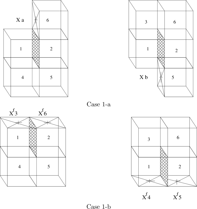

  

  Configuration with neighbor

• 2. Case 2: The neighbor cell is not available

  In the case shown in Fig. 4 (Case 2-a), ${\mathbf{X}}_{a}$ is replaced by the midpoint of the face on which we want to approach the flux (respectively ${\mathbf{X}}_{b}$). For the case shown in Fig. 4 (Case 2-b), ${\mathbf {X}}_{a}$ and ${\mathbf{X}}_{b}$ are respectively replaced by the midpoint of the faces that are at the top and in the lower part of the face.

  Figure 4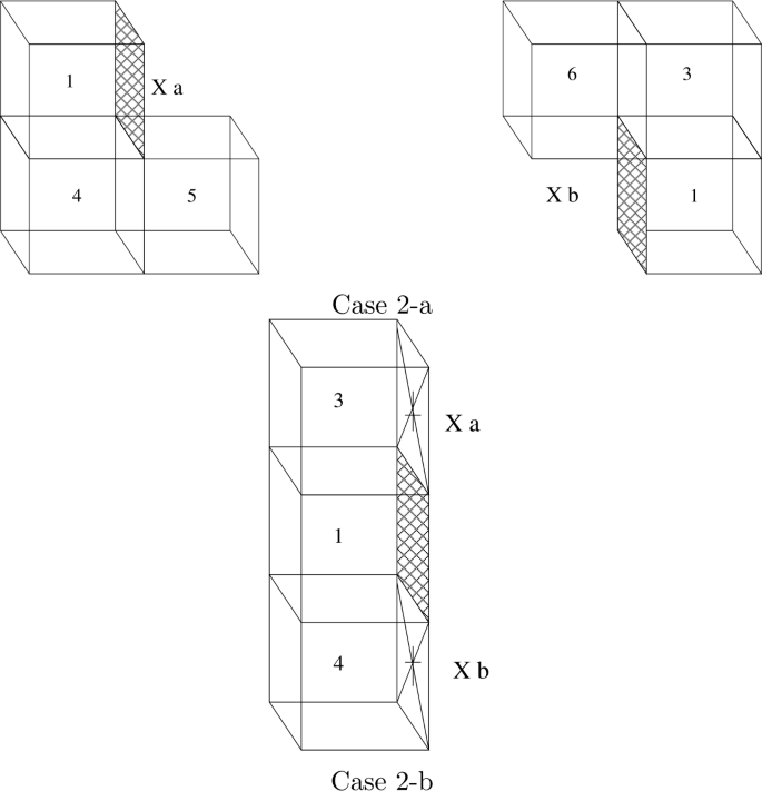

  

  Configuration without neighbor

Remark 3.1

In the treatment of the boundary conditions, we only presented how we construct the points ${\mathbf {X}}_{a}$ and ${\mathbf{X}}_{b}$. For the points ${\mathbf {X}}_{c}$ and ${\mathbf{X}}_{d}$, the construction is carried out in the same way.

4 Numerical validation

4.1 Numerical convection tests

To validate the convection part, we investigate the widely used tests in the literature: the shock tube problem introduced in [37] and the Lax test [38] in their 3D version. The domain is the unit cube and the considered mesh is 101 × 11 × 101. The time step is calculated using the Courant–Friedrichs–Lewy (CFL) condition: $\displaystyle \max _{1\leq k\leq 3}|\lambda _{k}| \frac{\triangle t}{\triangle x}<1$ ($\lambda _{k}$ is the wave-speed, $\triangle x =\min |F_{i^{+}}-F_{i^{-}}|$, $F_{i^{+}}$, $F_{i^{-}}$ are two adjacent faces of the cell $M_{i}$). At $t=0$, datum are respectively:

$$\begin{aligned}& {\text{shock tube: }}\quad (\rho ,{\mathbf{u}},p)= \left \{ \textstyle\begin{array}{l@{\quad}r@{\quad}r} 1.0,\;(0,0,0),\;1.0~~~~~~&{\text{if}}&~~~~ x< 0.5, \\ 0.1 ,\;(0,0,0),\;0.125~~~~~~&{\text{if}}&~~~~x>0.5, \end{array}\displaystyle \right . \end{aligned}$$

(14)

$$\begin{aligned}& {\text{Lax test: }} \quad (\rho ,{\mathbf{u}},p)= \left \{ \textstyle\begin{array}{l@{\quad}r@{\quad}r} 0.445,\;(0,0,0),\;3.528~~~~~~&{\text{if}}&~~~~ x< 0.5, \\ 0.5 ,\;(0,0,0),\;0.571~~~~~~&{\text{if}}&~~~~x>0.5. \end{array}\displaystyle \right . \end{aligned}$$

(15)

Figures 5 and 6 show the numerical solution in the middle of the cube, and one can see that we reproduce the expected results. However, some numerical diffusion appears mainly on the rarefaction. This is related to the Godunov scheme we use. Our goal in this part is primarily to use a more general state law given by (2).

Figure 5

3D Gary A. Sod test: Y = 0.5, Z = 0.5, CFL = 0.9, time = 0.15

Figure 6

3D Lax P D test: Y = 0.5, Z = 0.5, CFL = 0.9,time = 0.15

4.2 Numerical convection tests with boundary conditions

For resolution of the half Riemann problem, we use the initial datum (14), and to have different wave types, we impose various boundaries conditions given by (16).

$$\begin{aligned} {\mathbf{u}}_{b}= \left \{ \textstyle\begin{array}{l@{\quad}r@{\quad}r} (-0.2,0,0)_{a},\;(-0.2,0,0)_{b},\;(-0.9,0,0)_{c},\;(-0.9,0,0)_{d}&{ \text{if}}&x=0, \\ (-0.5,0,0)_{a},\;(0.5,0,0)_{b},\;(-0.5,0,0)_{c},\;(0.5,0,0)_{d}&{ \text{if}}&x=1. \end{array}\displaystyle \right . \end{aligned}$$

(16)

Figure 7 shows horizontal velocity profiles on which one can clearly see the effect of the boundary condition.

Figure 7

Velocity profile (Gary A. Sod test): Y = 0.5, Z = 0.5, CFL = 0.9

4.3 Diffusion validation tests

4.3.1 Scalar case

To validate the scalar case, we consider the following heat equation (17):

$$\begin{aligned} \textstyle\begin{array}{l} \left \{ \textstyle\begin{array}{l@{\quad}r@{\quad}r} \rho C_{v}\displaystyle \frac{\partial{ u}}{\partial t} -k \triangle u= 0&{\text{ in }}& [0,T]\times \Omega , \\ \displaystyle u(x=0,y,z,t)=u_{1} &{\text{ on }}&\Gamma _{1}, \\ u(x=L,y,z,t)= u_{2} &{\text{ on }}&\Gamma _{2}, \\ u= u_{1} + \frac{x}{L}(u_{2} - u_{1}) &{\text{ on }}&\Gamma _{3}. \end{array}\displaystyle \right . \end{array}\displaystyle \end{aligned}$$

(17)

We use the same time step as that calculated in the convection. The considered domain is $\Omega = [0,L]\times [0,L]\times [0,L]$ with boundary ∂Ω divided into three parts defined as follows:

$$ \displaystyle \Gamma _{1} = \displaystyle \left \lbrace x=0,\:(y,z) \in \mathbb{R}^{2} \right \rbrace ~,~ \displaystyle \Gamma _{2} = \displaystyle \left \lbrace x=L,\:(y,z)\in \mathbb{R}^{2} \right \rbrace {\text{, and}}~~ \displaystyle \Gamma _{3} = \partial \Omega \setminus \displaystyle \Gamma _{1}\cup \Gamma _{2}. $$

The exact solution is given by

$$ u^{\text{ex}}(x,y,z,t) = e^{-\frac{12\pi}{L^{2}}\frac{k}{\rho C_{v}}t} \sin (\frac{2\pi x}{L})\sin (\frac{2\pi y}{L})\sin (\frac{2\pi z}{L}) + u_{1} + \frac{x}{L}(u_{2} - u_{1}). $$

We consider two numerical test cases. On the one hand, a structured mesh with two different sizes, and on the other hand, a nonstructured one with three different sizes (see Fig. 8). Figures 9 and 10 show respectively the exact and obtained solutions for the structured and unstructured meshes. We obtain a good approximation for the different cases, and we remark that for the unstructured meshes, the obtained numerical solution is more accurate when the mesh size decreases. This is confirmed by the $L^{\infty}$ relative error obtained in Table 1 for the case of unstructured meshes.

Figure 8

Plane cut of the different used unstructured meshes

Figure 9

Structured case

Figure 10

Unstructured case

Table 1 $L^{\infty}$ relative error

4.3.2 Vector case

The vector case is studied in this section. We consider the same meshes as in the scalar test, but with a homogeneous Dirichlet boundary condition.

We consider the following problem:

$$ {\rho}\displaystyle \frac{\partial {\mathbf{u}}}{\partial t} - \mu \triangle {\mathbf{u}} -(\frac{\mu}{3}+\lambda )\nabla (\nabla \cdot {\mathbf{u}})=0, $$

whose exact solution is given by

$$ {\mathbf{u}}(t,x,y,z)=\displaystyle e^{- \frac{4\pi ^{2}(3\mu +\frac{\lambda}{3})t}{L^{2}}}\sin ( \displaystyle \frac{2\pi x}{L})\sin (\displaystyle \frac{2\pi y}{L}) \sin (\displaystyle \frac{2\pi z}{L}){\vec{\mathbf{e}}_{1}}. $$

Figure 11 shows the obtained $\mathrm{L}^{1}$ relative error for various meshes and times step.

Figure 11

$\mathrm{L}^{1}$ relative error

4.4 The natural convection test

To validate the complete Navier–Stokes system (1), we study the natural convection test (see [39]). The velocity is taken homogeneous on the boundary, and a temperature gradient is imposed between the left and right vertical boundaries. In Figs. 12 and 13, we represent respectively the obtained results for the temperature isovalues and velocity field, for various Rayleigh numbers (Ray), using mesh M3. The obtained results are in close agreement with the those in [39].

Figure 12

The temperature isovalues for different Ray numbers

Figure 13

Velocity field for different Ray numbers

4.5 Lid-driven test

The geometry of this problem is a square cavity. The boundary condition is ${\mathbf{u}}=(1,0,0)$ on the top, and homogeneous boundary conditions on all other sides. The obtained result in Fig. 14 is similar to the result given in [40, 41].

Figure 14

Lid-driven test

5 Conclusion

In this work, we present a new technique to solve the three-dimensional compressible Navier–Stokes system on unstructured mesh. A splitting method is used to solve separately the convection and the diffusion parts. The originality of our work is mainly to present a new scheme to approximate the diffusive flux, which can be used both on structured or unstructured mesh. The numerical validation tests show good accuracy of the developed scheme.

References

Wang, J., Jiang, H.: Time decay of solutions for compressible isentropic non-Newtonian fluids. Bound. Value Probl. 2024, 7 (2024)
Watanabe, K.: Stability of stationary solutions to the three-dimensional Navier-Stokes equations with surface tension. Adv. Nonlinear Anal. 12(1), 1–35 (2023)
Guo, Y., Sun, R., Wang, W.: Optimal time-decay rates of the Keller–Segel system coupled to compressible Navier–Stokes equation in three dimensions. Bound. Value Probl. 2022, 37 (2022)
Hammad, H.A., Aydi, H., Kattan, D.A.: Hybrid interpolative mappings for solving fractional Navier–Stokes and functional differential equations. Bound. Value Probl. 2023, 116 (2023)
Tong, L.: Global existence and decay estimates of the classical solution to the compressible Navier-Stokes-Smoluchowski equations in \(r^{3}\). Adv. Nonlinear Anal. 13(1), 1–25 (2024)
Abdelwahed, M., Chorfi, N., Mezghani, N., Ouertani, H.: An algorithm for solving the Navier–Stokes problem with mixed boundary conditions. Bound. Value Probl. 2022, 94 (2022)
Girault, V., Raviart, P.A.: Finite Element Approximation of the Navier–Stokes Equations, vol. 749. Springer, Berlin (1981)
Glowinski, R., Pironneau, O.: Finite element methods for Navier-Stokes equations. Annu. Rev. Fluid Mech. 24, 167–204 (1992)
Temam, R.: Sur L’approximation de la Solution des Equations de Navier–Stokes Par la Méthode des Pas Fractionnaires. North-Holland, Amsterdam (1984)
Abdelwahed, M., Chorfi, N.: Spectral discretization of the time-dependent Navier–Stokes problem with mixed boundary conditions. Adv. Nonlinear Anal. 11(1), 1447–1465 (2022)
Bernardi, C., Maday, Y.: Approximation Spectrales Pour les Problèmes aux Limites Elliptiques. Springer, Paris (1992)
Hussaini, M.Y., Canuto, C., Quarteroni, A., Zang, T.A.: Numerical Solutions for a Comparison Problem on Natural Convection in Enclosed Cavity. Springer, Berlin (1988)
Minev, P.D., Timmernans, L.J.P., Van De Vosse, F.N.: An approximate projection scheme for incompressible flow using spectral elements. Int. J. Numer. Methods Fluids 22, 673–688 (1996)
Boivin, S., Cayré, F., Hérard, J.M.: A finite volume method to solve the Navier–Stokes equations for incompressible flows on unstructured meshes. Int. J. Therm. Sci. 39, 806–825 (2000)
Boivin, S., Hérard, J.M., Perron, S.: A finite volume method to solve the 3d Navier-Stokes equations on unstructured collocated meshes. Comput. Fluids 33(10), 1305–1333 (2004)
Pironneau, O.: Méthodes des éléments Finis Pour les Fluides. Masson, Paris (1988)
Abboud, H., Sayah, T.: A full discretization of the time-dependent Navier-Stokes equations by a two-grid scheme. Math. Model. Numer. Anal. 42(1), 141–174 (2008)
Chorin, A.J.: Numerical solution of the Navier–Stokes equations. Math. Comput. 22, 745–762 (1968)
Jobelin, M., Piar, B., Angot, P., Latché, J.-C.: Une méthode de pénalité-projection pour les écoulements dilatables. Rev. Eur. Méc. Numér. 17(4), 453–480 (2008)
Eymard, R., Gallouët, T., Herbin, R.: A cell-centred finite volume approximation for anisotropic diffusion operators on unstructured meshes in any space dimension. IMA J. Numer. Anal. 26, 326–353 (2006)
Eymard, R., Gallouët, T., Herbin, R.: Finite Volume Methods, Handbook of Numerical Analysis. North Holland, Amsterdam (2000)
Domelevo, K., Omnes, P.: A finite volume scheme for the Laplace equation on almost arbitrary two-dimensional grids. Math. Model. Numer. Anal. 39(6), 1203–1249 (2005)
Manzini, G., Russo, A.: A finite volume method for advection diffusion problems in convection-dominated regimes. Comput. Methods Appl. Mech. Eng. 197, 1242–1261 (2008)
Jacques, M., Saurel, R., Nkonga, B., Abgrall, R.: Propositions de méthodes et modèles eulériens pour les problèmes à interfaces entre fluides compressibles en présence de transfert de chaleur. Int. J. Heat Mass Transf. 45(6), 1287–1307 (2002)
Abgrall, R., Saurel, R.: A simple method for compressible multiphase flows. SIAM J. Sci. Comput. 21(3), 1115–1145 (1999)
Andrainov, N., Richard, S.W.: A simple method for compressible multiphase mixture and interfaces. Rapport de recherche 4247, INRIA (2001)
Rouy, S.: Modélisation mathématique et numérique d’écoulement diphasique compressible. application au cas industriel d’un générateur de gaz. PhD thesis, Université de Toulou et du Var (2000)
Edwige, G., Raviart, P.A.: Numerical Approximation of Hyperbolic Systems of Conservation Laws. Collection Applied Mathematical Sciences. Springer, New York (1996)
Toro, E.F.: Riemann Solvers and Numerical Methods for Fluid Dynamics. Springer, Paris (1997)
Abdelwahed, M., Chorfi, N.: On the convergence analysis of a time dependent elliptic equation with discontinuous coefficients. Adv. Nonlinear Anal. 9(1), 1145–1160 (2020)
Serre, D.: Système de Lois de Conservation I. Springer, Paris (1996)
Villa, J.P.: Sur la théorie et l’approximation de problèmes hyperboliques non linéaires application aux équations de saint venant et à la modélisation des avalanches de neige dense. PhD thesis, Université de Paris VI (1986)
Dubois, F.: Résolution Numérique du Problème de Riemann, Polycopier du cours dea analyse numérique edn. Ecole Polytechnique, Université Paris V, Paris XIII. Ecole Polytechnique, Université Paris V
Kirkkörrü, K., Uygun, M.: Numerical solution of the Euler equations by finite volume methods: central versus upwind schemes. J. Aeronaut. Spaces Tech. 2(1), 47–55 (2005)
Chorfi, N., Abdelwahed, M., Berselli, C.: On the analysis of geometrically selective turbulence model. Adv. Nonlinear Anal. 9(1), 1402–1419 (2020)
Faille, I.: A control volume method to solve an elliptic equation on two-dimensional irregular mesh. Comput. Methods Appl. Mech. Eng. 100, 1992 (1992)
Gary, A.S.: A survey of several finite difference methods for systems of non-linear hyperbolic conservation law. J. Comput. Phys. 2, 1–31 (1978)
Lax, P.D.: Weak solutions of non-linear hyperbolic equations and their numerical approximation. Commun. Pure Appl. Math. 7, 159–193 (1954)
Jones, I.P., Thompson, P.: Numerical solutions for a comparison problem on natural convection in enclosed cavity. Technical report, Computer Science and Sys. Division, AERE Harwell (1981)
Djadel, K., Nicaise, S.: A non-conforming finite volume element method of weighted upstream type for the two-dimensional stationary Navier–Stokes system. Appl. Numer. Math. 58, 615–634 (2008)
Thomasset, F.: Implement of the Finite Element Method for Navier-Stokes Equations. Springer, Paris (1981)
Acknowledgements
Researchers Supporting Project number (RSP2024R136), King Saud University, Riyadh, Saudi Arabia.
Funding
Not applicable.
Author information
Authors and Affiliations
Contributions
The authors declare that the study was realized in collaboration with equal responsibility. All authors read and approved the final manuscript.
Corresponding author
Ethics declarations
Competing interests
The authors declare no competing interests.
Additional information
Publisher’s Note
Springer Nature remains neutral with regard to jurisdictional claims in published maps and institutional affiliations.
Rights and permissions
Open Access This article is licensed under a Creative Commons Attribution 4.0 International License, which permits use, sharing, adaptation, distribution and reproduction in any medium or format, as long as you give appropriate credit to the original author(s) and the source, provide a link to the Creative Commons licence, and indicate if changes were made. The images or other third party material in this article are included in the article’s Creative Commons licence, unless indicated otherwise in a credit line to the material. If material is not included in the article’s Creative Commons licence and your intended use is not permitted by statutory regulation or exceeds the permitted use, you will need to obtain permission directly from the copyright holder. To view a copy of this licence, visit http://creativecommons.org/licenses/by/4.0/.
About this article
Cite this article
Abdelwahed, M., Bade, R., Chaker, H. et al. On the study of three-dimensional compressible Navier–Stokes equations. Bound Value Probl 2024, 84 (2024). https://doi.org/10.1186/s13661-024-01893-9
Received:
Accepted:
Published:
DOI: https://doi.org/10.1186/s13661-024-01893-9