- Research Article
- Open access
- Published:
Global Behavior for a Diffusive Predator-Prey Model with Stage Structure and Nonlinear Density Restriction-I: The Case in 
Boundary Value Problems volume 2009, Article number: 378763 (2009)
Abstract
This paper deals with a Holling type III diffusive predator-prey model with stage structure and nonlinear density restriction in the space  . We first consider the asymptotical stability of equilibrium points for the model of ODE type. Then, the existence and uniform boundedness of global solutions and stability of the equilibrium points for the model of weakly coupled reaction-diffusion type are discussed. Finally, the global existence and the convergence of solutions for the model of cross-diffusion type are investigated when the space dimension is less than 6.
1. Introduction
Population models with stage structure have been investigated by many researchers, and various methods and techniques have been used to study the existence and qualitative properties of solutions [1–9]. However, most of the discussions in these works are devoted to either systems of ODE or weakly coupled systems of reaction-diffusion equations. In this paper we investigate the global existence and convergence of solutions for a strongly coupled cross-diffusion predator-prey model with stage structure and nonlinear density restriction. Nonlinear problems of this kind are quite difficult to deal with since the usual idea to apply maximum principle arguments to get priori estimates cannot be used here [10].
Consider the following predator-prey model with stage-structure:

where  ,
,  denote the density of the immature and mature population of the prey, respectively,
  is the density of the predator. For the prey, the immature population is nonlinear density restriction.
  is assumed to consume
  with Holling type III functional response
  and contributes to its growth with rate
  . For more details on the backgrounds of this model see references [11, 12].
Using the scaling  and redenoting
  by
by  , we can reduce the system (1.1) to

where 
To take into account the natural tendency of each species to diffuse, we are led to the following PDE system of reaction-diffusion type:

where  is a bounded domain in
  with smooth boundary
  ,
,  is the outward unit normal vector on
  , and
, and  .
.  are nonnegative smooth functions on
  . The diffusion coefficients
  are positive constants. The homogeneous Neumann boundary condition indicates that system (1.3) is self-contained with zero population flux across the boundary. The knowledge for system (1.3) is limited (see [13–17]).
In the recent years there has been considerable interest to investigate the global behavior for models of interacting populations with linear density restriction by taking into account the effect of self-as well as cross-diffusion [18–26]. In this paper we are led to the following cross-diffusion system:

where  are the diffusion rates of the three species, respectively.
  are referred as self-diffusion pressures, and
  is cross-diffusion pressure. The term self-diffusion implies the movement of individuals from a higher to a lower concentration region. Cross-diffusion expresses the population fluxes of one species due to the presence of the other species. The value of the cross-diffusion coefficient may be positive, negative, or zero. The term positive cross-diffusion coefficient denotes the movement of the species in the direction of lower concentration of another species and negative cross-diffusion coefficient denotes that one species tends to diffuse in the direction of higher concentration of another species [27]. For
  , problem (1.4) becomes strongly coupled with a full diffusion matrix. As far as the authors are aware, very few results are known for cross-diffusion systems with stage-structure.
The main purpose of this paper is to study the asymptotic behavior of the solutions for the reaction-diffusion system (1.3), the global existence, and the convergence of solutions for the cross-diffusion system (1.4). The paper will be organized as follows. In Section 2 a linear stability analysis of equilibrium points for the ODE system (1.2) is given. In Section 3 the uniform bound of the solution and stability of the equilibrium points to the weakly coupled system (1.3) are proved. Section 4 deals with the existence and the convergence of global solutions for the strongly coupled system (1.4).
2. Global Stability for System (1.2)
Let  . If
. If  , then (1.2) has semitrivial equilibria
  , where
  . To discuss the existence of the positive equilibrium point of (1.2), we give the following assumptions:

where  . Let one curve
  :
:  , and the other curve
  :
:  . Obviously,
  passes the point
  . Noting that
  attains its maximum at
  , thus when
  ,
,  .
.  has the asymptote
  and passes the point
  . In this case,
  and
and  have unique intersection
  , as shown in Figure 1.
 is the unique positive equilibrium point of (1.2), where
  ,
,  ,
,  . In addition, the restriction of the existence of the positive equilibrium can be removed, if
  .
.

Figure 1
The Jacobian matrix of the equilibrium  is
is

The characteristic equation of  (
( ) is
) is  .
.  is a saddle for
  . In addition, the dimensions of the local unstable and stable manifold of
  are 1 and 2, respectively.
  is locally asymptotically stable for
  .
.
The Jacobian matrix of the equilibrium  is
is

where  . The characteristic equation of
  (
( ) is
) is  , where

According to Routh-Hurwitz criterion,  is locally asymptotically stable for
  and
and  , that is,
  and
and  .
.
The Jacobian matrix of the equilibrium  is
is

where

The characteristic equation of  (
( ) is
) is  , where

According to Routh-Hurwitz criterion,  is locally asymptotically stable for
  . Obviously,
  can be checked by (2.1).
Now we discuss the global stability of equilibrium points for (1.2).
Theorem 2.1.
-
(i)
Assume that (2.1),
 (2.8)
(2.8)

hold, then the equilibrium point  of (1.2) is globally asymptotically stable.
-
(ii)
Assume that
 , and
, and  hold, then the equilibrium point
  of (1.2) is globally asymptotically stable.
 -
(iii)
Assume that
 holds, then the equilibrium point
  of (1.2) is globally asymptotically stable.
 , and
, and  hold, then the equilibrium point
  of (1.2) is globally asymptotically stable.
 holds, then the equilibrium point
  of (1.2) is globally asymptotically stable.
Proof.
-
(i)
Define the Lyapunov function
 (2.9)
(2.9)

Calculating the derivative of  along the positive solution of (1.2), we have

When  , the minimum of
  and
and  is
is  and 0, respectively; the maximum of
  is
is  are
are  and
and  , respectively. Thus, when (2.8) hold,
  According to the Lyapunov-LaSalle invariance principle [28],
  is globally asymptotically stable if (2.1)–(2.3) hold.
-
(ii)
Let
 (2.11)

Then

Noting that the maximum of  is
is  , and
, and  , we find
  . Therefore,
-
(iii)
Let
 (2.13)

then

Thus,  for
for  . This completes the proof of Theorem 2.1.
3. Global Behavior of System (1.3)
In this section we discuss the existence, uniform boundedness of global solutions, and the stability of constant equilibrium solutions for the weakly coupled reaction-diffusion system (1.3). In particular, the unstability results in Section 2 also hold for system (1.3) because solutions of (1.2) are also solutions of (1.3).
Theorem 3.1.
Let  be nonnegative smooth functions on
  . Then system (1.3) has a unique nonnegative solution
  , and
, and

on  . In particular, if
  , then
  for all
  .
.
Proof.
It is easily seen that  is sufficiently smooth in
  and possesses a mixed quasimonotone property in
  . In addition,
  and
and  are a pair of lower-upper solutions of problem (1.3) (cf.
  in (3.1)). From [29, Theorem 5.3.4], we conclude that (1.3) exists a unique classical solution
  satisfying (3.1). According to strong maximum principle, it follows that
  . So the proof of the Theorem is completed.
Remark 3.2.
When  (namely
  ), system (1.3) reduces to a system in which the immature population of the prey is linear density restriction. Similar to the proof of Theorem 3.1, we have

Now we show the local and global stability of constant equilibrium solutions  for (1.3), respectively.
Theorem 3.3.
-
(i)
Assume that (2.1) holds, then the equilibrium point
 of (1.3) is locally asymptotically stable.
 -
(ii)
Assume that
 ,
,  , and
, and  hold, then the equilibrium point
  of (1.3) is locally asymptotically stable.
 -
(iii)
Assume that
 holds, then the equilibrium point
  of (1.3) is locally asymptotically stable.
 of (1.3) is locally asymptotically stable.
 ,
,  , and
, and  hold, then the equilibrium point
  of (1.3) is locally asymptotically stable.
 holds, then the equilibrium point
  of (1.3) is locally asymptotically stable.
Proof.
Let  be the eigenvalues of the operator
  on
on  with Neumann boundary condition, and let
  be the eigenspace corresponding to
  in
in  . Let
. Let

where  is an orthonormal basis of
  , then

 Let
Let  ,
,  , where

The linearization of (1.3) is  at
at  . For each
  ,
,  is invariant under the operator L, and
  is an eigenvalue of L on
  , if and only if
  is an eigenvalue of the matrix
  . The characteristic equation is
  , where

From Routh-Hurwitz criterion, we can see that three eigenvalues (denoted by  ,
,  ,
,  ) all have negative real parts if and only if
  . Noting that
  , we must have
  . It is easy to check that
  if
if  (see Section 2).
We can conclude that there exists a positive constant  , such that

In fact, let  , then

Since  as
as  , it follows that

Clearly,  has the three roots
  . Let
. Let  . By continuity, there exists
  such that the three roots
  of
of  satisfy

Let  , then
  . Let
. Let  , then (3.7) holds. According to [30, Theorem 5.1.1], we have the locally asymptotically stability of
  .
.
-
(ii)
The linearization of (1.4) is
 at
at  , where
  , and
, and 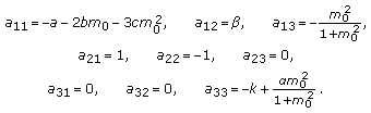 (3.11)
 at
at  , where
  , and
, and 
The characteristic equation of  is
is  , where

The three roots of  all have negative real parts for
  and
and  . Namely,
  is the locally asymptotically stable, if
  and
and  .
.
-
(iii)
The linearization of (1.3) is
 at
at  , where
  , and
, and 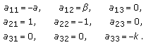 (3.13)
 at
at  , where
  , and
, and 
Similar to (i),  is locally asymptotically stable, when
  .
.
Remark 3.4.
When  denote
  . If
. If  , then (1.3) has the semitrivial equilibrium point
  , where
  . If
. If  , then (1.3) has a unique positive equilibrium point
  . Similar as Theorem 3.3, we have the following.
(i)If  ,
,  , and
, and  (namely,
  ,
,  ,
,  ), then
  is locally asymptotically stable.
(ii)If  and
and  , then
  is locally asymptotically stable.
(iii)If  , then
  is locally asymptotically stable.
Before discussing the global stability, we give an important lemma which has been proved in [31, Lemma  ] or in [32, Lemma
  ].
].
Lemma 3.5.
Let  be positive constants. Assume that
  ,
,  , and
, and  is bounded from below. If
  and
and  for some positive constant
  , then
Theorem 3.6.
-
(i)
Assume that (2.1),
 (3.14)

hold, then the equilibrium point  of system (1.3) is globally asymptotically stable.
-
(ii)
Assume that
 , and
, and  hold, then the equilibrium point
  of system (1.3) is globally asymptotically stable.
 , and
, and  hold, then the equilibrium point
  of system (1.3) is globally asymptotically stable.
(iii)Assume that  and
and  hold, then the equilibrium point
  of system (1.3) is globally asymptotically stable.
Proof.
Let  be the unique positive solution of (1.3). By Theorem 3.1, there exists a positive constant C which is independent of
  and
and  such that
  , for
, for  . By [33, Theorem
  ],
],

-
(i)
Define the Lyapunov function
 (3.16)

By Theorem 3.1,  is defined well for all solutions of (1.3) with the initial functions
  . It is easily see that
  and
and  if and only if
  .
.
Calculating the derivative of  along positive solution of (1.3) by integration by parts and the Cauchy inequality, we have

It is not hard to verify that

if (3.14) hold. Applying Lemma 3.5, we can obtain

Recomputing  , we find

From (3.15), we can see that  is bounded in
  ,
,  . It follows from Lemma 3.5 and (3.15) that
  as
as  . Namely,

Using the Pioncaré inequality, we have

where  Noting that

according to (3.19) and (3.22), we can see

Thus, there exists  as
as  . Applying the boundness of
  , there exists a subsequence of
  , denoted still by
  , such that
  On the one hand

On the other hand

According to (3.19) to compute the limit of the previous equation and using the uniqueness of the limit, we have  , and
, and

It follows from (3.15) that there exists a subsequence of  , denoted still by
  , and nonnegative functions
  , such that

Applying (3.19)–(3.27), we obtain that  , and
, and

In view of Theorem 3.3, we can conclude that  is globally asymptotically stable.
-
(ii)
Let
 (3.30)

Then

Therefore,  It follows that the equilibrium point
  of (1.3) is globally asymptotically stable.
-
(iii)
Define
 (3.32)

Then

When  ,
,

The following proof is similar to (i).
Remark 3.7.
When  , Theorem 3.6 shows the following.
-
(i)
Assume that
 ,
,  (3.35)
 ,
, 
hold, then the equilibrium point  of (1.3) is globally asymptotically stable.
-
(ii)
Assume that
 hold, then the equilibrium point
  of (1.3) is globally asymptotically stable.
 -
(iii)
Assume that
 and
and  hold, then the equilibrium point
  of (1.3) is globally asymptotically stable.
 hold, then the equilibrium point
  of (1.3) is globally asymptotically stable.
 and
and  hold, then the equilibrium point
  of (1.3) is globally asymptotically stable.
Example 3.8.
Consider the following system:

Using the software Matlab, one can obtain  ,
,  . It is easy to see that the previous system satisfies the all conditions of Theorem 3.6(i). So the positive equilibrium point (0.5637,0.5637,0.1199) of the previous system is globally asymptotically stable.
4. Global Existence and Stability of Solutions for the System (1.4)
By [34–36], we have the following result.
Theorem 4.1.
If  , then (1.4) has a unique nonnegative solution
  , where
  is the maximal existence time of the solution. If the solution
  satisfies the estimate

then  . If, in addition,
  , then
In this section, we consider the existence and the convergence of global solutions to the system (1.4).
Theorem 4.2.
Let  and the space dimension
  . Suppose that
  are nonnegative functions and satisfy zero Neumann boundary conditions. Then (1.4) has a unique nonnegative solution
In order to prove Theorem 4.2, some preparations are collected firstly.
Lemma 4.3.
Let  be a solution of (1.4). Then

where  .
.
Proof.
From the maximum principle for parabolic equations, it is not hard to verify that  and
and  is bounded.
Multiplying the second equation of (1.4) by  , adding up the first equation of (1.4), and integrating the result over
  , we obtain

Using Young inequality and H lder inequality, we have

where  It follows from (4.3) and (4.4) that

Thus,

where  depends on
  and coefficients of (1.4). In addition, there exists a positive constant
  , such that

Integrating the first equation of (1.4) over  , we have

Integrating (4.8) from  to
to  , we have

According to (4.7), there exists a positive constant  , such that

Multiplying the second equation of (1.4) by  and integrating it over
  , we obtain

Integrating the previous inequation from  to
to  , we have

Lemma 4.4.
Let  be a solution of (1.4),
  , and
, and  . Then there exists a positive constant
  depending on
  and
and  , such that

Furthermore  and
and 
Proof.
 satisfies the equation

where  are functions of
  and so are bounded because of Lemma 4.3.
Multiply the second equation of (1.4) by  and integrate it over
  to obtain

Then

and  . From a disposal similar to the proof of Lemma 2.2 in [23], we have
  . Using a standard embedding result, we obtain
Lemma 4.5 (see [23, Lemmas 2.3 and 2.4]).
Let  ,
,  , and let
  be any number which may depend on
  . Then there is a constant
  depending on
  , and
, and  such that

for any  with
with  for all
  .
.
To obtain  -estimates of
  , we establish
  -estimates of
  in the following lemma.
Lemma 4.6.
Let  ,
,  , then there exist positive constants
  and
and  , such that

Proof.
Multiply the first equation of (1.4) by  for
for  and integrate by parts over
  to obtain

Integrating (4.19) from 0 to  , we have

Then substitution of  ,
,  into (4.20) leads to

It follows from H lder inequality and Lemma 4.3 that

Note that  , and
, and  for
for  . From H
 lder inequality, Young inequality, and Lemma 4.4, we have

Substitution of (4.22) and (4.23) into (4.21) leads to

where  is arbitrary and
  .
.
Choose  such that

then it follows from (4.24) that

Let

Then  for
for

According to Lemma 4.5 and the definition of  , we can see

Combining (4.26) and (4.29), we have

where  . Therefore
  is bounded from (4.30).
From (4.29), we have  . Namely,
  ,
,  . Combining (4.28), we have
  , where
  .
.
Setting  in (4.20) (it is easily checked that
  , i.e.,
  ), we have
  .
.
Multiplying the second equation of (1.4) by  and integrating it over
  , we have

The result of  can be obtained from an analogue of the previous proof of
  's.
's.
Lemma 4.7.
Let  , then there exists a positive constant
  such that

Proof.
We will prove this lemma by [37, Theorem 7.1, page 181]. At first, we rewrite the first two equations of (1.4) as

where  ,
,  ,
,  ,
,  is
is  symbol. It follows from Lemma 4.6 that
  ,
,  .
.
By the third equation of (1.4), we have

It follows from Lemma 4.3 that  is bounded in
  . Applying Theorem
  [37, Page 204] to (4.34), we have

Recall that  satisfy (4.14) in Lemma 4.4, that is,

where  is bounded. Since
  by (4.35), applying Theorem
  [37, page 341-342] to (4.36), we have

It follows from [37, Lemma  , page 80] that
  and so
  . Recall from Lemma 4.6 that
  , so that
  by applying Theorem
  [37, Page 181] to (4.33).
Proof of Theorem 4.2.
Firstly, Theorem 4.2 can be proved in a similar way as Theorem  in [21, 25] when the space dimension
  .
.
Secondly, for  , applying Lemma
  [37, Page 80] to (4.36), we have

Since  , we obtain

The first two equations can be written in the divergence form as

where  . It follows from Lemmas 4.1, 4.5, and (4.39) that
  are bounded. Thus applying Theorem
  [37, Page 204] to (4.40) leads to

We rewrite the third equation of (1.4) as

where  . Applying Schauder estimate [29, Theorem
  , page 114] to (4.42) gives

Let

then

where  ,
,  . From (4.41), we have
  . It follows from (4.41) and (4.43) that
  . Applying Schauder estimate to (4.45) gives

Solving equations (4.44) for  , respectively, we have

In particular, to conclude  , we need to repeat the above bootstrap technique. Since
  is arbitrary, so the classical solution
  of (1.4) exists globally in time.
Now we discuss the global stability of the positive equilibrium  (see Section 2) for (1.4).
Theorem 4.8.
Assume that the all conditions in Theorem 4.2, (2.1), and

hold. Let  be the unique positive equilibrium point of (1.4), and let
  be a positive solution for (1.4). Then

provided that  is large enough.
Proof.
Define the Lyapunov function

Let  be a positive solution of (1.4), Then

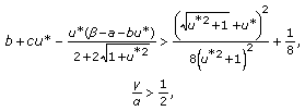
The first integrand in the right hand of the previous inequality is positive definite if

Therefore, when the all conditions in Theorem 4.8 hold, there exists a positive constant  such that

This implies that  . So the proof of Theorem 4.8 is completed.
References
Aiello WG, Freedman HI: A time-delay model of single-species growth with stage structure. Mathematical Biosciences 1990, 101(2):139–153. 10.1016/0025-5564(90)90019-U
Zhang X, Chen L, Neumann AU: The stage-structured predator-prey model and optimal harvesting policy. Mathematical Biosciences 2000, 168(2):201–210. 10.1016/S0025-5564(00)00033-X
Liu S, Chen L, Liu Z: Extinction and permanence in nonautonomous competitive system with stage structure. Journal of Mathematical Analysis and Applications 2002, 274(2):667–684. 10.1016/S0022-247X(02)00329-3
Lin Z: Time delayed parabolic system in a two-species competitive model with stage structure. Journal of Mathematical Analysis and Applications 2006, 315(1):202–215. 10.1016/j.jmaa.2005.06.012
Xu R: A reaction-diffusion predator-prey model with stage structure and nonlocal delay. Applied Mathematics and Computation 2006, 175(2):984–1006. 10.1016/j.amc.2005.08.014
Xu R, Chaplain MAJ, Davidson FA: Global convergence of a reaction-diffusion predator-prey model with stage structure for the predator. Applied Mathematics and Computation 2006, 176(1):388–401. 10.1016/j.amc.2005.09.028
Xu R, Chaplain MAJ, Davidson FA: Global convergence of a reaction-diffusion predator-prey model with stage structure and nonlocal delays. Computers & Mathematics with Applications 2007, 53(5):770–788. 10.1016/j.camwa.2007.02.002
Wang M: Stability and Hopf bifurcation for a prey-predator model with prey-stage structure and diffusion. Mathematical Biosciences 2008, 212(2):149–160. 10.1016/j.mbs.2007.08.008
Wang Z, Wu J: Qualitative analysis for a ratio-dependent predator-prey model with stage structure and diffusion. Nonlinear Analysis: Real World Applications 2008, 9(5):2270–2287. 10.1016/j.nonrwa.2007.08.004
Galiano G, Garzón ML, Jüngel A: Semi-discretization in time and numerical convergence of solutions of a nonlinear cross-diffusion population model. Numerische Mathematik 2003, 93(4):655–673. 10.1007/s002110200406
Chen L: Mathematical Models and Methods in Ecology. Science Press, Beijing, China; 1988.
Chen LJ, Sun JH: The uniqueness of a limit cycle for a class of Holling models with functional responses. Acta Mathematica Sinica 2002, 45(2):383–388.
Li W-T, Wu S-L: Traveling waves in a diffusive predator-prey model with Holling type-III functional response. Chaos, Solitons & Fractals 2008, 37(2):476–486. 10.1016/j.chaos.2006.09.039
Ko W, Ryu K: Qualitative analysis of a predator-prey model with Holling type II functional response incorporating a prey refuge. Journal of Differential Equations 2006, 231(2):534–550. 10.1016/j.jde.2006.08.001
Zhang H, Georgescu P, Chen L: An impulsive predator-prey system with Beddington-DeAngelis functional response and time delay. International Journal of Biomathematics 2008, 1(1):1–17. 10.1142/S1793524508000072
Fan Y, Wang L, Wang M: Notes on multiple bifurcations in a delayed predator-prey model with nonmonotonic functional response. International Journal of Biomathematics 2009, 2(2):129–138. 10.1142/S1793524509000583
Wang F, An Y: Existence of nontrivial solution for a nonlocal elliptic equation with nonlinear boundary condition. Boundary Value Problems 2009, 2009:-8.
Lou Y, Ni W-M: Diffusion, self-diffusion and cross-diffusion. Journal of Differential Equations 1996, 131(1):79–131. 10.1006/jdeq.1996.0157
Lou Y, Ni W-M, Wu Y: On the global existence of a cross-diffusion system. Discrete and Continuous Dynamical Systems 1998, 4(2):193–203.
Shim S-A: Uniform boundedness and convergence of solutions to cross-diffusion systems. Journal of Differential Equations 2002, 185(1):281–305. 10.1006/jdeq.2002.4169
Shim S-A: Uniform boundedness and convergence of solutions to the systems with cross-diffusions dominated by self-diffusions. Nonlinear Analysis: Real World Applications 2003, 4(1):65–86. 10.1016/S1468-1218(02)00014-7
Choi YS, Lui R, Yamada Y: Existence of global solutions for the Shigesada-Kawasaki-Teramoto model with weak cross-diffusion. Discrete and Continuous Dynamical Systems 2003, 9(5):1193–1200.
Choi YS, Lui R, Yamada Y: Existence of global solutions for the Shigesada-Kawasaki-Teramoto model with strongly coupled cross-diffusion. Discrete and Continuous Dynamical Systems 2004, 10(3):719–730.
Pang PYH, Wang MX: Existence of global solutions for a three-species predator-prey model with cross-diffusion. Mathematische Nachrichten 2008, 281(4):555–560. 10.1002/mana.200510624
Fu S, Wen Z, Cui S: Uniform boundedness and stability of global solutions in a strongly coupled three-species cooperating model. Nonlinear Analysis: Real World Applications 2008, 9(2):272–289. 10.1016/j.nonrwa.2006.10.003
Yang F, Fu S: Global solutions for a tritrophic food chain model with diffusion. The Rocky Mountain Journal of Mathematics 2008, 38(5):1785–1812. 10.1216/RMJ-2008-38-5-1785
Dubey B, Das B, Hussain J: A predator-prey interaction model with self and cross-diffusion. Ecological Modelling 2001, 141(1–3):67–76.
Hale JK: Ordinary Differential Equations. Krieger, Malabar, Fla, USA; 1980.
Ye Q, Li Z: Introduction to Reaction-Diffusion Equations. Science Press, Beijing, China; 1999.
Henry D: Geometric Theory of Semilinear Parabolic Equations, Lecture Notes in Mathematics. Volume 840. Springer, Berlin, Germany; 1993.
Lin Z, Pedersen M: Stability in a diffusive food-chain model with Michaelis-Menten functional response. Nonlinear Analysis: Theory, Methods & Applications 2004, 57(3):421–433. 10.1016/j.na.2004.02.022
Wang M: Nonliear Parabolic Equation of Parabolic Type. Science Press, Beijing, China; 1993.
Brown KJ, Dunne PC, Gardner RA: A semilinear parabolic system arising in the theory of superconductivity. Journal of Differential Equations 1981, 40(2):232–252. 10.1016/0022-0396(81)90020-6
Amann H: Dynamic theory of quasilinear parabolic equations. I. Abstract evolution equations. Nonlinear Analysis: Theory, Methods & Applications 1988, 12(9):895–919. 10.1016/0362-546X(88)90073-9
Amann H: Dynamic theory of quasilinear parabolic equations. II. Reaction-diffusion systems. Differential and Integral Equations 1990, 3(1):13–75.
Amann H: Dynamic theory of quasilinear parabolic systems. III. Global existence. Mathematische Zeitschrift 1989, 202(2):219–250. 10.1007/BF01215256
Ladyženskaja OA, Solonnikov VA, Ural'ceva NN: Linear and Quasilinear Equations of Parabolic Type, Translations of Mathematical Monographs. Volume 23. American Mathematical Society, Providence, RI, USA; 1967:xi+648.
Acknowledgments
This work has been partially supported by the China National Natural Science Foundation (no. 10871160), the NSF of Gansu Province (no. 096RJZA118), the Scientific Research Fund of Gansu Provincial Education Department, and NWNU-KJCXGC-03-47 Foundation.
Author information
Authors and Affiliations
Corresponding author
Rights and permissions
Open Access This article is distributed under the terms of the Creative Commons Attribution 2.0 International License ( https://creativecommons.org/licenses/by/2.0 ), which permits unrestricted use, distribution, and reproduction in any medium, provided the original work is properly cited.
About this article
Cite this article
Zhang, R., Guo, L. & Fu, S. Global Behavior for a Diffusive Predator-Prey Model with Stage Structure and Nonlinear Density Restriction-I: The Case in  .
Bound Value Probl 2009, 378763 (2009). https://doi.org/10.1155/2009/378763
.
Bound Value Probl 2009, 378763 (2009). https://doi.org/10.1155/2009/378763
Received:
Accepted:
Published:
DOI: https://doi.org/10.1155/2009/378763