Hierarchies of Difference Boundary Value Problems

Abstract

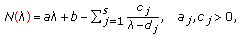
This paper generalises the work done in Currie and Love (2010), where we studied the effect of applying two Crum-type transformations to a weighted second-order difference equation with various combinations of Dirichlet, non-Dirichlet, and affine -dependent boundary conditions at the end points, where is the eigenparameter. We now consider general -dependent boundary conditions. In particular we show, using one of the Crum-type transformations, that it is possible to go up and down a hierarchy of boundary value problems keeping the form of the second-order difference equation constant but possibly increasing or decreasing the dependence on of the boundary conditions at each step. In addition, we show that the transformed boundary value problem either gains or loses an eigenvalue, or the number of eigenvalues remains the same as we step up or down the hierarchy.

1. Introduction

Our interest in this topic arose from the work done on transformations and factorisations of continuous Sturm-Liouville boundary value problems by Binding et al. [1] and Browne and Nillsen [2], notably. We make use of analogous ideas to those discussed in [3–5] to study difference equations in order to contribute to the development of the theory of discrete spectral problems.

Numerous efforts to develop hierarchies exist in the literature, however, they are not specifically aimed at difference equations per se and generally not for three-term recurrence relations. Ding et al., [6], derived a hierarchy of nonlinear differential-difference equations by starting with a two-parameter discrete spectral problem, as did Luo and Fan [7], whose hierarchy possessed bi-Hamiltonian structures. Clarkson et al.'s, [8], interest in hierarchies lay in the derivation of infinite sequences of systems of difference equations by using the Bcklund transformation for the equations in the second Painlev equation hierarchy. Wu and Geng, [9], showed early on that the hierarchy of differential-difference equations possesses Hamiltonian structures while a Darboux transformation for the discrete spectral problem is shown to exist.

In this paper, we consider a weighted second-order difference equation of the form

(1.1)

where represents a weight function and a potential function.

Our aim is to extend the results obtained in [10, 11] by establishing a hierarchy of difference boundary value problems. A key tool in our analysis will be the Crum-type transformation (2.1). In [10], it was shown that (2.1) leaves the form of the difference equation (1.1) unchanged. For us, the effect of (2.1) on the boundary conditions will be crucial. We consider (eigenparameter)-dependent boundary conditions at the end points. In particular, the eigenparameter dependence at the initial end point will be given by a positive Nevanlinna function, say, and at the terminal end point by a negative Nevanlinna function, say. The case of was covered in [10] and the the case of constant was studied in [11]. Applying transformation (2.1) to the boundary conditions results in a so-called transformed boundary value problem, where either the new boundary conditions have more -dependence, less -dependence, or the same amount of -dependence as the original boundary conditions. Consequently the transformed boundary value problem has either one more eigenvalue, one less eigenvalue, or the same number of eigenvalues as the original boundary value problem. Thus, it is possible to construct a chain, or hierarchy, of difference boundary value problems where the successive links in the chain are obtained by applying the variations of (2.1) given in this paper. For instance, it is possible to go from a boundary value problem with -dependent boundary conditions to a boundary value problem with -independent boundary conditions or vice versa simply by applying the correct variation of (2.1) an appropriate number of times. Moreover, at each step, we can precisely track the eigenvalues that have been lost or gained. Hence, this paper provides a significant development in the theory of three-term difference boundary value problems in regard to singularities and asymptotics in the hierarchy structure. For similar results in the continuous case, see [12].

There is an obvious connection between the three-term difference equation and orthogonal polynomials. In fact, the three-term recurrence relation satisfied by orthogonal polynomials is perhaps the most important information for the constructive and computational use of orthogonal polynomials [13].

Difference equations and operators and results concerning their existence and construction of their solutions have been discussed in [14, 15]. Difference equations arise in numerous settings and have applications in diverse areas such as quantum field theory, combinatorics, mathematical physics and biology, dynamical systems, economics, statistics, electrical circuit analysis, computer visualization, and many other fields. They are especially useful where recursive computations are required. In particular see [16] [9, Introduction] for three physical applications of the difference equation (1.1), namely, the vibrating string, electrical network theory and Markov processes, in birth and death processes and random walks.

It should be noted that G. Teschl's work, [17, Chapter  11], on spectral and inverse spectral theory of Jacobi operators, provides an alternative factorisation, to that of [10], of a second-order difference equation, where the factors are adjoints of one another.

This paper is structured as follows.

In Section 2, all the necsessary results from [10] are recalled, in particular how (1.1) transforms under (2.1). In addition, we also recap some important properties of Nevanlinna functions.

The focus of Section 3 is to show exactly the effect that (2.1) has on boundary conditions of the form

(1.2)

We give explicitly the new boundary conditions which are obeyed, from which it can be seen whether the -dependence has increased, decreased, or remained the same.

Lastly, in Section 4, we compare the spectrum of the original boundary value problem with that of the transformed boundary value problem and show under which conditions the transformed boundary value problem has one more eigenvalue, one less eigenvalue, or the same number of eigenvalues as the original boundary value problem.

2. Preliminaries

In [10], we considered (1.1) for , where the values of and are given by boundary conditions, that is, is defined for .

Let the mapping be defined by

(2.1)

where, throughout this paper, is a solution to (1.1) for such that for all . Whether or not obeys the various given boundary conditions (to be specified later) is of vital importance in obtaining the results that follow.

From [10], we have the following theorem.

Theorem 2.1.

Under the mapping (2.1), (1.1) transforms to

(2.2)

where for

(2.3)

We now recall some properties of Nevanlinna functions.

• (I) The inverse of a positive Nevanlinna function is a negative Nevanlinna function, that is

  

  (2.4)

where are positive Nevanlinna functions. This follows directly from the fact that if and only if .

• (II) If

  

  (2.5)

then

(2.6)

This follows by (I) together with the fact that since has zeros has poles. Also as so as . Thus, if is a positive Nevanlinna function of the form (2.5), then for , is a negative Nevanlinna function of the same form.

• (III) If

  

  (2.7)

then

(2.8)

since has zeros so has poles and as so as .

For the remainder of the paper, will denote a Nevanlinna function where

is the number of terms in the sum;

indicates the value of at which the boundary condition is imposed and

(2.9)

3. General -Dependent Boundary Conditions

In this section, we show how obeying general -dependent boundary conditions transforms, under (2.1), to obeying various types of -dependent boundary conditions. The exact form of these boundary conditions is obtained by considering the number of zeros and poles (singularities) of the various Nevanlinna functions under discussion and these correlations are illustrated in the different graphs depicted in this section.

Lemma 3.1.

If obeys the boundary condition

(3.1)

then the domain of may be extended from to by forcing the condition

(3.2)

where

(3.3)

with .

Proof.

The transformed equation (2.2), for , together with (3.2) gives

(3.4)

Also the mapping (2.1), together with (3.1), yields

(3.5)

Substituting (3.5) into (3.4), we obtain

(3.6)

Now (2.1), with , gives

(3.7)

which when substituted into (3.6) and dividing through by results in

(3.8)

This may be rewritten as

(3.9)

Using (1.1), with , together with (3.1), gives

(3.10)

Subtracting (3.10) from (3.9) results in

(3.11)

Rearranging the above equation and dividing through by yields

(3.12)

and hence

(3.13)

Thus obeys the equation on the extended domain.

The remainder of this section illustrates why it is so important to distinguish between the two cases of obeying or not obeying the boundary conditions.

Theorem 3.2.

Consider obeying the boundary condition (3.1) where is a positive Nevanlinna function, that is, for . Under the mapping (2.1), obeying (3.1) transforms to obeying (3.2) as follows.

If does not obey (3.1) then obeys

(3.14)

(3.15)

If does obey (3.1) for then obeys

(3.16)

(3.17)

where , that is, are positive Nevanlinna functions.

In (A) and (B), is not possible.

Proof.

The fact that is by construction, see Lemma 3.1. We now examine the form of in Lemma 3.1. Let , , and then

(3.18)

But

(3.19)

thus

(3.20)

Now has the expansion

(3.21)

where and the 's correspond to where , that is, the singularities of (3.20).

Since is a positive Nevanlinna function it has a graph of the form shown in Figure 1.

Clearly, the gradient of at is positive for all , that is,

(3.22)

If does not obey (3.1), then the zeros of

(3.23)

are the poles of , that is, the 's and where for . It is evident, from Figure 1, that the number of 's is equal to the number of 's, thus in (3.21), .

We now examine the form of in (3.21). As it follows that . Thus

(3.24)

Therefore

(3.25)

Hence, substituting into (3.20) gives

(3.26)

Let

(3.27)

Then since , and we have that and clearly if then giving (3.14), that is,

(3.28)

If then we want so that we have a positive Nevanlinna function, that is

(3.29)

which means that either,

(3.30)

giving that, since ,

(3.31)

which is as shown in Figure 1, or,

(3.32)

giving that

(3.33)

but this means that which is not possible.

Thus, for , that is, given , the ratio must be chosen suitably to ensure that is a positive Nevanlinna function as required. Hence we obtain (3.15), that is

(3.34)

If obeys (3.1), for , then . Thus in Figure 1, one of the 's is equal to and since is less than the least eigenvalue of the boundary value problem (1.1), (3.1) together with a boundary condition at (specified later) it follows that , as for all .

Now

(3.35)

and as

(3.36)

Thus is a removable singularity. Alternatively,

(3.37)

which illustrates that the singularity at is removable.

We now have that the number of nonremovable singularities, , in (3.20) is one less than the number of 's , see Figure 1. Thus (3.21) becomes

(3.38)

which may be rewritten as

(3.39)

where , for .

We now examine the form of in (3.39). As , we have that, as before, . Thus

(3.40)

Hence, from (3.20),

(3.41)

Let

(3.42)

Then since , and we have that and clearly if then giving (3.16), that is,

(3.43)

If then we need so that we have a positive Nevanlinna function, that is

(3.44)

which means that either

(3.45)

giving that, since ,

(3.46)

which is as shown in Figure 1, or,

(3.47)

giving that

(3.48)

but this means that which is not possible.

Thus, for , that is, given , the ratio must be chosen suitably to ensure that is a positive Nevanlinna function as required. Hence, we obtain (3.17), that is,

(3.49)

Figure 1

.

In the theorem below, we increase the dependence by introducing a nonzero term in the original boundary condition. As in Theorem 3.2, the dependence of the transformed boundary condition depends on whether or not obeys the given boundary condition. In addition, to ensure that the dependence of the transformed boundary condition is given by a positive Nevanlinna function it is necessary that the transformed boundary condition is imposed at 0 and 1 as opposed to −1 and 0. Thus the interval under consideration shrinks by one unit at the initial end point. By routine calculation it can be shown that the form of the dependence of the transformed boundary condition, if imposed at −1 and 0, is neither a positive Nevalinna function nor a negative Nevanlinna function.

Theorem 3.3.

Consider obeying the boundary condition

(3.50)

where is a positive Nevanlinna function, that is, and for . Under the mapping (2.1), obeying (3.50) transforms to obeying the following.

(1) If does not obey (3.50) then obeys

(3.51)

(2) If does obey (3.50), for , then obeys

(3.52)

where .

Proof.

Since and are defined we do not need to extend the domain in order to impose the boundary conditions (3.51) or (3.52).

The mapping (2.1), at , together with (3.50) gives

(3.53)

Also (2.1), at , is

(3.54)

Substituting in for from (1.1), with , and using (3.50), we obtain that

(3.55)

From (3.53) and (3.55), it now follows that

(3.56)

As in Theorem 3.2, let and . Then (3.56) becomes

(3.57)

From Theorem 3.2, we have that so

(3.58)

Also, as in Theorem 3.2,

(3.59)

has the expansion

(3.60)

where corresponds to , that is, the singularities of (3.59). Now is a positive Nevanlinna function with graph given in Figure 2.

Clearly, the gradient of at is positive for all , that is,

(3.61)

If does not obey (3.50) then the zeros of

(3.62)

are the poles of , that is, the 's and where for . It is evident, from Figure 2, that the number of 's is one more than the number of 's, thus in (3.60), .

We now examine the form of in (3.60). As it follows that , thus

(3.63)

Hence, .

Using (3.58) we now obtain

(3.64)

Note that . Let

(3.65)

then

(3.66)

Now since if then , that is, but and so this is not possible. Therefore by Section 2, Nevanlinna result (II), we have that

(3.67)

that is, (3.51) holds.

If does obey (3.50) for then . Thus, in Figure 2, one of the 's, is equal to and since is less than the least eigenvalue of the boundary value problem (1.1), (3.50) together with a boundary condition at (specified later) it follows that , as for all .

Now (3.59) can be written as

(3.68)

and as

(3.69)

Thus is a removable singularity. Alternatively, we could substitute in for and to illustrate that the singularity at is removable, see Theorem 3.2. Hence the number of nonremovable 's is the same as the number of 's, see Figure 2. So (3.60) becomes

(3.70)

which may be rewritten as

(3.71)

where and for .

We now examine the form of in (3.70). As , we have that , thus

(3.72)

Hence, . So, from (3.58) with , we obtain

(3.73)

where, as before,

(3.74)

Thus, by Section 2, Nevanlinna result (II), we have that

(3.75)

that is, (3.52) holds.

Figure 2

.

In Theorem 3.4, we impose a boundary condition at the terminal end point and show how it is transformed according to whether or not obeys the given boundary condition.

Theorem 3.4.

Consider obeying the boundary condition at given by

(3.76)

where is a negative Nevanlinna function, that is, and for . Under the mapping (2.1), obeying (3.76) transforms to obeying the following.

(I) If does not obey (3.76) then obeys

(3.77)

(II) If does obey (3.76) then obeys

(3.78)

where .

Proof.

Since and are defined we do not need to extend the domain of in order to impose the boundary conditions (3.77) or (3.78).

The mapping (2.1), at , gives

(3.79)

From (1.1), with , we can substitute in for in the above equation to get

(3.80)

Using (3.76), we obtain

(3.81)

But obeys (1.1) at , for , so that (3.81) becomes

(3.82)

Also, for , (2.1) together with (3.76) yields

(3.83)

Therefore,

(3.84)

Let , then (3.84) may be rewritten as

(3.85)

By Section 2, Nevanlinna result (I), since is a negative Nevanlinna function it follows that is a positive Nevanlinna function, which has the form

(3.86)

by Section 2, Nevanlinna result (III).

As before has expansion

(3.87)

where , , corresponds to the singularities of (3.85), that is, where . The graph of is as shown in Figure 3.

As before, the gradient of at is positive for all , that is

(3.88)

If does not obey (3.76) then the zeros of

(3.89)

are the poles of , that is, the 's and where for . Clearly, from Figure 3, the number of 's is the same as the the number of 's, thus in (3.87), .

Next, we examine the form of in (3.87). As it follows that . Thus

(3.90)

Therefore, . Hence,

(3.91)

where , , and for , which is precisely (3.77).

If does obey (3.76) for then . Thus in Figure 3, one of the 's, is equal to and since is less than the least eigenvalue of the boundary value problem (1.1), (3.76) together with a boundary condition at −1 (as given in Theorems 3.2 or 3.3) it follows that , as for all .

Now

(3.92)

and as

(3.93)

Thus is a removable singularity. Again, alternatively, we could have substituted in for and to illustrate that the singularity at is removable, see Theorem 3.2. Hence the number of nonremovable 's is one less than the number of 's, see Figure 3.

So (3.87) becomes

(3.94)

which may be rewritten as

(3.95)

where and for .

Now as ,

(3.96)

So, we obtain

(3.97)

where , , , and for all , that is, we obtain (3.78).

Figure 3

.

4. Comparison of the Spectra

In this section, we investigate how the spectrum of the original boundary value problem compares to the spectrum of the transformed boundary value problem. This is done by considering the degree of the eigenparameter polynomial for the various eigenconditions.

Lemma 4.1.

Consider the boundary value problem given by (1.1) for together with boundary conditions

(4.1)

(4.2)

Then the boundary value problem (1.1), (4.1), (4.2) has eigenvalues. (Note that the number of unit intervals considered is .)

Proof.

From (1.1), with , we obtain

(4.3)

Substituting in for from (4.1) yields

(4.4)

which may be rewritten as

(4.5)

where , are real constants.

Now (1.1), for , together with (4.5) results in

(4.6)

where , are real constants.

Thus, by induction,

(4.7)

for real constants , . Similarly

(4.8)

for real constants , .

Since , using boundary condition (4.2) we obtain the following eigencondition:

(4.9)

where , , are real constants.

Thus, the numerator is a polynomial, in , of order . Note that, none of the roots of this polynomial are given by , or , since, from Figures 1 to 3, it is easy to see that none of the eigenvalues of the boundary value problem are equal to the poles of the boundary conditions. Also is not a problem as the curve of the Nevanlinna function never intersects with the horizontal or oblique asymptote. This means that there are no common factors to cancel out. Hence the eigencondition has roots giving that the boundary value problem has eigenvalues.

As a direct consequence of Theorems 2.1, 3.2, 3.3, 3.4, and Lemma 4.1 we have the following theorem.

Theorem 4.2.

For the original boundary value problem we consider twelve cases, (see Table 1 in the Appendix), each of which has s+l+m+1 eigenvalues. The corresponding transformed boundary value problem for each of the twelve cases, together with the number of eigenvalues for that transformed boundary value problem, is given in Table 1 (see the appendix).

Table 1 Table 1

Remark 4.3.

To summarise we have the following.

• (a) If obeys the boundary conditions at both ends the transformed boundary value problem will have one less eigenvalue than the original boundary value problem, namely, .

• (b) If obeys the boundary condition at one end only the transformed boundary value problem will have the same eigenvalues as the original boundary value problem.

• (c) If does not obey any of the boundary conditions the transformed boundary value problem will have one more eigenvalue than the original boundary value problem, namely, .

Corollary 4.4.

If are the eigenvalues of any one of the original boundary value problems (1)–(9), in Theorem 4.2, with corresponding eigenfunctions then

(i) are the eigenvalues of the corresponding transformed boundary value problems (1)–(3), in Theorem 4.2, with corresponding eigenfunctions ;

(ii) are the eigenvalues of the corresponding transformed boundary value problems (4)–(9), in Theorem 4.2, with corresponding eigenfunctions .

Also, if are the eigenvalues of any one of the original boundary value problems (10)–(12), in Theorem 4.2, with corresponding eigenfunctions then are the eigenvalues of the corresponding transformed boundary value problems (10)–(12), in Theorem 4.2, with corresponding eigenfunctions .

Proof.

By Theorems 2.1, 3.2, 3.3, and 3.4, we have that (2.1) transforms eigenfunctions of the original boundary value problems (1)–(9) to eigenfunctions of the corresponding transformed boundary value problems. In particular, if are the eigenvalues of one of the original boundary value problems, (1)–(9), with eigenfunctions then

(i) are the eigenfunctions of the corresponding transformed boundary value problem, (1)–(3), with eigenvalues . Since the transformed boundary value problems, (1)–(3), have eigenvalues it follows that constitute all the eigenvalues of the transformed boundary value problem;

(ii) are the eigenfunctions of the corresponding transformed boundary value problem, (4)–(9), with eigenvalues . Since the transformed boundary value problems, (4)–(9), have eigenvalues it follows that constitute all the eigenvalues of the transformed boundary value problem.

Also, again by Theorems 2.1, 3.2, 3.3, and 3.4, we have that (2.1) transforms eigenfunctions of the original boundary value problems (10)–(12) to eigenfunctions of the corresponding transformed boundary value problems. In particular, if are the eigenvalues of one of the original boundary value problems, (10)–(12), with eigenfunctions then are the eigenfunctions of the corresponding transformed boundary value problem, (10)–(12), with eigenvalues . Since the transformed boundary value problems, (10)–(12), have eigenvalues it follows that constitute all the eigenvalues of the transformed boundary value problem.

Twelve Cases for Theorem 4.2

See Table 1.

References

Binding PA, Browne PJ, Watson BA: Spectral isomorphisms between generalized Sturm-Liouville problems. In Linear Operators and Matrices, Operator Theory: Advances and Applications. Volume 130. Birkhäuser, Basel, Switzerland; 2002:135-152.
Browne PJ, Nillsen RV: On difference operators and their factorization. Canadian Journal of Mathematics 1983, 35(5):873-897. 10.4153/CJM-1983-050-2
Binding PA, Browne PJ, Watson BA: Sturm-Liouville problems with boundary conditions rationally dependent on the eigenparameter. II. Journal of Computational and Applied Mathematics 2002, 148(1):147-168. 10.1016/S0377-0427(02)00579-4
Binding PA, Browne PJ, Watson BA: Sturm-Liouville problems with reducible boundary conditions. Proceedings of the Edinburgh Mathematical Society. Series II 2006, 49(3):593-608. 10.1017/S0013091505000131
Binding PA, Browne PJ, Watson BA: Transformations between Sturm-Liouville problems with eigenvalue dependent and independent boundary conditions. Bulletin of the London Mathematical Society 2001, 33(6):749-757. 10.1112/S0024609301008177
Ding H-Y, Sun Y-P, Xue F-C: A hierarchy of differential-difference equations, conservation laws and new integrable coupling system. Communications in Nonlinear Science and Numerical Simulation 2010, 15(8):2037-2043. 10.1016/j.cnsns.2009.08.022
Luo L, Fan E-G: A hierarchy of differential-difference equations and their integrable couplings. Chinese Physics Letters 2007, 24(6):1444-1447. 10.1088/0256-307X/24/6/005
Clarkson PA, Hone ANW, Joshi N: Hierarchies of difference equations and Bäcklund transformations. Journal of Nonlinear Mathematical Physics 2003, 10(supplement 2):13-26. 10.2991/jnmp.2003.10.s2.2
Wu Y, Geng X: A new hierarchy of integrable differential-difference equations and Darboux transformation. Journal of Physics A 1998, 31(38):L677-L684. 10.1088/0305-4470/31/38/004
Currie S, Love AD: Transformations of difference equations I. Advances in Difference Equations 2010, 2010:-22.
Currie S, Love AD: Transformations of difference equations II. Advances in Difference Equations 2010, 2010:-23.
Binding PA, Browne PJ, Watson BA: Sturm-Liouville problems with boundary conditions rationally dependent on the eigenparameter. I. Proceedings of the Edinburgh Mathematical Society. Series II 2002, 45(3):631-645.
Gautschi W: Orthogonal Polynomials: Computation and Approximation, Numerical Mathematics and Scientific Computation. Oxford University Press, New York, NY, USA; 2004:x+301.
Miller KS: Linear Difference Equations. W. A. Benjamin, New York, NY, USA; 1968:x+105.
Miller KS: An Introduction to the Calculus of Finite Differences and Difference Equations. Dover, New York, NY, USA; 1966:viii+167.
Atkinson FV: Discrete and Continuous Boundary Problems, Mathematics in Science and Engineering. Volume 8. Academic Press, New York, NY, USA; 1964:xiv+570.
Teschl G: Jacobi Operators and Completely Integrable Nonlinear Lattices, Mathematical Surveys and Monographs. Volume 72. American Mathematical Society, Providence, RI, USA; 2000:xvii+351.
Acknowledgments
The authors would like to thank Professor Bruce A. Watson for his useful input. S. Currie is supported by NRF Grant nos. TTK2007040500005 and FA2007041200006.
Author information
Authors and Affiliations
Corresponding author
Additional information
An erratum to this article is available at http://dx.doi.org/10.1186/1687-2770-2012-66.