- Research Article
- Open access
- Published:
Existence Results of Three-Point Boundary Value Problems for Second-order Ordinary Differential Equations
Boundary Value Problems volume 2011, Article number: 901796 (2011)
Abstract
We establish existence results of the following three-point boundary value problems:  ,
,  ,
,  and
and  , where
  and
and  . The approach applied in this paper is upper and lower solution method associated with basic degree theory or Schauder's fixed point theorem. We deal with this problem with the function
  which is Carathéodory or singular on its domain.
1. Introduction
In this paper, we consider three-point boundary value problem


where  and
and  .
.
In the mathematical literature, a number of works have appeared on nonlocal boundary value problems, and one of the first of these was [1]. Il'in and Moiseev initiated the research of multipoint boundary value problems for second-order linear ordinary differential equations, see [2, 3], motivated by the study [4–6] of Bitsadze and Samarskii.
Recently, nonlinear multipoint boundary value problems have been receiving considerable attention, and have been studied extensively by using iteration scheme (e.g., [7]), fixed point theorems in cones (e.g., [8]), and the Leray-Schauder continuation theorem (e.g., [9]). We refer more detailed treatment to more interesting research [10, 11] and the references therein.
The theory of upper and lower solutions is also a powerful tool in studying boundary value problems. For the existence results of two-point boundary value problem, there already are lots of interesting works by applying this essential technique (see [12, 13]). Recently, it is shown that this method plays an important role in proving the existence of solutions for three-point boundary value problems (see [14–16]).
Last but not least, as the singular source term appearing in two-point problems, singular three-point boundary value problems also attract more attention (e.g., [17]).
In this paper, we will discuss the existence of solutions of some general types on three-point boundary value problems by using upper and lower solution method associated with basic degree theory or Schauder's fixed point theorem.
This paper is organized as follows. In Section 2, we give two lemmas which will be extensively used later. In Section 3, when the source term  is a Carathéodory function, we consider the Sobolev space
  defined by

and obtain the existence of  -solution in Theorems 3.5 and 3.11. In Section 4, we discuss the singular case, that is,
  maybe singular at the end points
  or
or  , or at
  . We will introduce the
  -class of functions and another space
  (see [18, 19]) as follows:

and prove the existence of  -solution in Theorems 4.1 and 4.4. Some sufficient conditions for constructing upper and lower solutions are given in each section for applications.
2. Preliminaries
Define  by
by

where  and
and  are given as (1.2) and

By direct computations, we get the following results.
Lemma 2.1.
-
(i)
The function
 defined by (2.1), is the Green function corresponding for the problem
 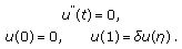 (2.3)
(2.3)
 defined by (2.1), is the Green function corresponding for the problem
(ii) The function  defined by (2.1), is continuous.
-
(iii)
In the case
 , we have
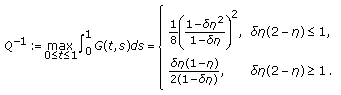 (2.4)
(2.4)
 , we have
Lemma 2.2.
If  , then the problem

with boundary condition (1.2) has a unique solution  such that

where  is defined by (2.1).
3. Carathéodory Case
In this section we first introduce the Carathéodory function as follows.
Definition 3.1.
A function  defined on
  is called a Carathéodory function on
  if
if
(i)for almost every 
 is continuous on
  ;
;
(ii)for any  the function
  is measurable on
  ;
;
(iii)for any  , there exists
  such that for any
  and for almost every
  with
with  , we have
  .
.
We in this section assume that  is a Carathéodory function and discuss the existence of
  -solution by assuming the existence of upper and lower solutions.
3.1. Existence of  -Solutions
 -Solutions
We first introduce the definitions of  -upper and lower solutions as below.
Definition 3.2.
A function  is called a
  -lower solution of problem (1.1) and (1.2) if it satisfies
(i) ,
,  , and
, and
(ii)for any  , either
  , or there exists an open interval
  containing
  such that
  and, for almost every
  , we have

Definition 3.3.
A function  is called a
  -upper solution of problem (1.1) and (1.2) if it satisfies
(i) ,
,  , and
, and
(ii)for any  , either
  , or there exists an open interval
  containing
  such that
  and, for almost every
  , we have

Before proving our main results, we first consider such a modified problem given as follows:

with boundary condition (1.2), where  is defined by

Proposition 3.4.
Let  and
and  be respective
  -lower and upper solutions of problem (1.1) and (1.2) with
  on
on  . If
. If  is a solution of problem (3.3) and (1.2), then
  , for any
  .
.
Proof.
Suppose there exists  such that

Case 1.
If  , we have
  , which implies
  Hence, by Definition 3.2 and the continuity of
  at
at  , there exist an open interval
  with
with  ,
,  and a neighborhood
  of
of  contained in
  such that for almost every
  ,
,

Furthermore, it follows from  that for
  ,
,  , we have

This implies that the minimum of  cannot occur at
  , a contradiction.
Case 2.
If  , by the definition of
  -lower solution
  , we then have

And we get a contradiction.
Case 3.
If  , it follows from the conclusion of Case 1 that

which is impossible.
Consequently, we obtain  on
on  . By the similar arguments as above, we also have

Theorem 3.5.
Let  and
and  be
be  -lower and upper solutions of problem (1.1) and (1.2) such that
  on
on  and let
  be a Carathéodory function on
  , where

Then problem (1.1) and (1.2) has at least one solution  such that, for all
  ,
,

Proof.
We consider the modified problem (3.3) and (1.2) with respect to the given  and
and  . Consider the Banach space
  with supremum and the operator
  by
by

for  , where
  is defined as (2.1). Since
  is a Carathéodory function on
  , for almost all
  and for all
  , there exists a function
  , we have

Define

where


It is clear that  is a closed, bounded and convex set in
  and one can show that
  is a completely continuous mapping by Arzelà-Ascoli theorem and Lebesgue dominated convergence theorem. By applying Schauder's fixed point theorem, we obtain that
  has a fixed point in
  which is a solution of problem (3.3) and (1.2). From Proposition 3.4, this fixed point is also a solution of problem (1.1) and (1.2). Hence, we complete the proof.
We further illustrate the use of Theorem 3.11 in the following second-order differential equation:

with the boundary condition (1.2).
Corollary 3.6.
Assume that  is a Carathéodory function satisfying
  is essentially bounded for
  , where
  is a constant large enough. Assume further that
  and there exists a constant
  such that

Then, problem (3.18) and (1.2) has at least one solution.
Proof.
By hypothesis, for any given  small enough such that
  and for almost all
  , for any
  large enough, we have

We now choose an upper solution  of the form

To this end, we compute

Clearly, one can choose  such that

that is,

and choose  , where
  , which is a positive solution of

Hence, if  is large enough, we can show that
  and
and  , where
  , which implies that
  is a positive
  -upper solution. In the same way we construct a
  -lower solution
  on
on  .
.
3.2. Nontangency Solution
In this subsection, we afford another stronger lower and upper solutions to get a strict inequality of the solution between them.
Definition 3.7.
A function  is a strict
  -lower solution of problem (1.1) and (1.2), if it is not a solution of problem (1.1) and (1.2),
  ,
,  and for any
  , one of the following is satisfied:
(i) ;
;
(ii)there exist an interval  and
and  such that
  int
int ,
,  and for almost every
  , for all
  we have

Definition 3.8.
A function  is a strict
  -upper solution of problem (1.1) and (1.2), if it is not a solution of problem (1.1) and (1.2),
  ,
,  and for any
  , one of the following is satisfied:
(i) ,
,
(ii)there exist an interval  and
and  such that
  int
int ,
,  and for almost every
  , for all
  we have

Remark 3.9.
Every strict  -lower(upper) solution of problem (1.1) and (1.2) is a
  -lower(upper) solution.
Now we are going to show that the solution curve of problem (1.1) and (1.2) cannot be tangent to upper or lower solutions from below or above.
Proposition 3.10.
Let  and
and  be respective strict
  -lower and upper solutions of problem (1.1) and (1.2) with
  on
on  . If
. If  is a solution of problem (1.1) and (1.2) with
  on
on  , then
  , for any
  .
.
Proof.
As  is not a solution,
  is not identical to
  . Assume, the conclusion does not hold, then

exists. Hence,  has minimum at
  , that is,
  .
.
Case 1.
Set  . Since
  has minimum at
  , we have
  . According to the Definition 3.7, there exist
  ,
,  and
and  with
with  such that, for every
  ,
,  ,
,  and for a.e.

Hence, we have the contradiction since

Case 2.
If  , by the definition of strict
  -lower solution that
  , we then have

And we get a contradiction.
Case 3.
If  , repeat the same arguments in Case 3 of the proof of Proposition 3.4. Therefore, we obtain
  on
on  . The inequality
  on
on  can be proved by the similar arguments as above.
Theorem 3.11.
Let  and
and  be strict
  -lower and upper solutions of problem (1.1) and (1.2) such that
  on
on  and let
  be a Carathéodory function, where

Then, problem (1.1) and (1.2) has at least one solution  such that, for any
  ,
,

Proof.
This is a consequence of Theorem 3.5 and Proposition 3.10 and hence, we omits this proof.
4. Singular Case
In this section we give a more general existence result than Theorem 3.11 by assuming the existence of  -lower and upper solutions. This makes us to deal with problem (1.1) and (1.2), where the function
  is singular at the end point
  and
and  .
.
Theorem 4.1.
Let  and
and  be
be  -lower and upper solutions of problem (1.1) and (1.2) such that
  on
on  and let
  satisfy the following conditions:
(i)for almost every 
 is continuous on
  ;
;
(ii)for any  the function
  is measurable on
  ;
;
(iii)there exists a function  such that, for all
  ,
,

where

Then problem (1.1) and (1.2) has at least one solution  such that, for all
  ,
,

Proof.
Consider the modified problem (3.3) and (1.2) with respect to the given  and
and  and define
  by (3.13). Note that by Lemma 2.2,
  is well defined. Define

where

and  is defined by (3.17). The rest arguments are similar to the proof of Theorem 3.5.
Remark 4.2.
We have similar results of Theorems 3.5–4.1, respectively, for (1.1) equipped with

where  is a constant and
  ,
,  are given as (1.2).
Example 4.3.
Consider the problem (4.7), for  ,
,  ,
,  ,
,

Clearly,  is a
is a  -lower solution of (4.7) and

where

From Lemma 2.1, we have  and define
  . Since, for
  ,
, 

that is,  , we have, from Lemma 2.2,
  and
and  exists. Let

and, by Lemma 2.2 again, choose  such that

Note that according to the direct computation, we see that  is well-defined and is bounded by
  . Next, let
  . By Young's inequality, it follows that

Hence, such  is a
is a  -upper solution of (4.7) and
  on
on  . Clearly,
  satisfies (i), (ii) of Theorem 4.1. By using Young's inequality again, for
  , we have

and  . Therefore,
  satisfies the assumption (iii) of Theorem 4.1. Consequently, we conclude that this problem has at least one solution
  such that, for all
  ,
,

Notice that in Theorem 4.1, one can only deal with the case that  is singular at end points
  ,
,  . However, when
  is singular at
  , there is no hope to obtain the solutions directly from Theorem 4.1. We will establish the following theorem to deal with this case by constructing upper and lower solutions to solve this problem.
Theorem 4.4.
Assume
the function  is continuous;
there exists  and for any compact set
  , there is
  such that

for some  and
and  , there is
  such that

where  is defined as in Lemma 2.1.
for any compact set  , there is
  such that

Then problem (1.1) and (1.2) with  has at least one solution

Remark 4.5 (see [12, Remark  ]).
]).
Assumption  is equivalent to the assumption that there exists
  and a function
  such that:
(i) for all
  ,
,
(ii) , for all
  ,
,  ,
,
(iii) , for all
  ,
,
where

Proof.
Step 1.
Construction of lower solutions. Consider  such that
  and the function

where  is chosen small enough so that

Next, we choose  from the Remark 4.5, and let

where  is small enough so that for some points
  ,
,  , we have:


Notice that by (4.24) and (4.25), for any  such that

we have:


Step 2.
Approximation problems. We define for each  ,
,  ,
,

and set

We have that, for each index  ,
,  is continuous and

where

Hence, the sequence of functions  converges to
  uniformly on any set
  , where
  is an arbitrary compact subset of
  . Next we define

Each of the functions  is a continuous function defined on
  , moreover

and the sequence  converges to
  uniformly on the compact subsets of
  since
since

Define now a decreasing sequence  such that

and consider a sequence of the following approximation problems:

where  .
.
Step 3.
A lower solution of ( ). It is clear that for any  ,
,

As the sequence  is decreasing, we also have

Clearly,  satisfies

It follows from (4.25) and (4.27) that  is a lower solution of ( ).
Step 4.
Existence of a solution  of (4.7) such that

From assumption  , we can find
  and
and  such that, for all
  ,
,  ,
,

Also, one has

where  is a suitable constant. Hence, we obtain, for such
  and
and  ,
,

Let  be a constant such that

Choose  such that

that is,

where  is defined by (2.1). Note that
  is well-defined and
  since
since  . It is easy to see that

So by Remark 4.2, there is a solution  of (4.7) such that

Step 5.
The problem ( ) has at least one solution  such that

Notice that  is an upper solution of ( ), since

Step 6.
Existence of a solution. Consider the pointwise limit

It is clear that, for any  ,
,

and therefore  on
on  . Let
. Let  be a compact interval. There is an index
  such that
  for all
  and therefore for these
  ,
,

Moreover, we have

By Arzelá-Ascoli theorem it is standard to conclude that  is a solution of problem (1.1) and (1.2) on the interval
  . Since
  is arbitrary, we find that
  and for all
  ,
,

Since

it remains only to check the continuity of  at
at  . This can be deduced from the continuity of
  and the fact that
  as
as  .
.
Example 4.6.
Consider the following problem  , for
, for  ,
, ,
,  ,
,

Let  , where
  . Obviously,
  satisfies
  and
and  . Moreover, for any given
  and for any compact set
  , for
, for  small enough, we have

Hence,  holds. Furthermore, for
  large enough,
  , we have, from Young's inequality by choosing
  and
and  ,
,

where  . Hence,
  holds. By Theorem 4.4,
  has at least one solution

References
Bitsadze AV, Samarskii AA: On some of the simplest generalizations of linear elliptic boundary-value problems. Doklady Akademii Nauk SSSR 1969, 185: 739–740.
Il'in VA, Moiseev EI: Nonlocal boundary value problem of the first kind for a Sturm-Liouville operator in its differential and finite difference aspects. Differential Equations 1987, 23(7):803–810.
Il'in VA, Moiseev EI: Nonlocal boundary value problem of the second kind for a Sturm-Liouville operator. Differential Equations 1987, 23(7):979–987.
Bitsadze AV: On the theory of nonlocal boundary value problems. Soviet Mathematics—Doklady 1984, 30(1):8–10.
Bitsadze AV: On a class of conditionally solvable nonlocal boundary value problems for harmonic functions. Soviet Mathematics—Doklady 1985, 31(1):91–94.
Bitsadze AV, Samarskii AA: On some simple generalizations of linear elliptic boundary problems. Soviet Mathematics—Doklady 1969, 10(2):398–400.
Yao Q: Successive iteration and positive solution for nonlinear second-order three-point boundary value problems. Computers & Mathematics with Applications 2005, 50(3–4):433–444. 10.1016/j.camwa.2005.03.006
Yao Q: On the positive solutions of a second-order three-point boundary value problem with Caratheodory function. Southeast Asian Bulletin of Mathematics 2004, 28(3):577–585.
Gupta CP, Trofimchuk SI: A sharper condition for the solvability of a three-point second order boundary value problem. Journal of Mathematical Analysis and Applications 1997, 205(2):586–597. 10.1006/jmaa.1997.5252
Ma R: Positive solutions of a nonlinear m -point boundary value problem. Computers & Mathematics with Applications 2001, 42(6–7):755–765. 10.1016/S0898-1221(01)00195-X
Thompson HB, Tisdell C: Three-point boundary value problems for second-order, ordinary, differential equations. Mathematical and Computer Modelling 2001, 34(3–4):311–318. 10.1016/S0895-7177(01)00063-2
De Coster C, Habets P: Upper and lower solutions in the theory of ODE boundary value problems: classical and recent results. In Nonlinear Analysis and Boundary Value Problems for Ordinary Differential Equations, CISM Courses and Lectures. Volume 371. Edited by: Zanolin F. Springer, Vienna, Austria; 1993:1–78.
Lü H, O'Regan D, Agarwal RP: Upper and lower solutions for the singular p -Laplacian with sign changing nonlinearities and nonlinear boundary data. Journal of Computational and Applied Mathematics 2005, 181(2):442–466. 10.1016/j.cam.2004.11.037
Du Z, Xue C, Ge W: Multiple solutions for three-point boundary value problem with nonlinear terms depending on the first order derivative. Archiv der Mathematik 2005, 84(4):341–349. 10.1007/s00013-004-1196-7
Khan RA, Webb JRL: Existence of at least three solutions of a second-order three-point boundary value problem. Nonlinear Analysis. Theory, Methods & Applications 2006, 64(6):1356–1366. 10.1016/j.na.2005.06.040
Minghe P, Chang SK: The generalized quasilinearization method for second-order threepoint boundary value problems. Nonlinear Analysis. Theory, Methods & Applications 2008, 68(9):2779–2790. 10.1016/j.na.2007.02.025
Qu WB, Zhang ZX, Wu JD: Positive solutions to a singular second order three-point boundary value problem. Applied Mathematics and Mechanics 2002, 23(7):854–866. 10.1007/BF02456982
De Coster C, Habets P: Two-Point Boundary Value Problems: Lower and Upper Solutions. Springer, Berlin, Germany; 1984.
Habets P, Zanolin F: Upper and lower solutions for a generalized Emden-Fowler equation. Journal of Mathematical Analysis and Applications 1994, 181(3):684–700. 10.1006/jmaa.1994.1052
Author information
Authors and Affiliations
Corresponding author
Rights and permissions
Open Access This article is distributed under the terms of the Creative Commons Attribution 2.0 International License (https://creativecommons.org/licenses/by/2.0), which permits unrestricted use, distribution, and reproduction in any medium, provided the original work is properly cited.
About this article
Cite this article
Wang, SP., Tsai, LY. Existence Results of Three-Point Boundary Value Problems for Second-order Ordinary Differential Equations. Bound Value Probl 2011, 901796 (2011). https://doi.org/10.1155/2011/901796
Received:
Revised:
Accepted:
Published:
DOI: https://doi.org/10.1155/2011/901796