- Research
- Open access
- Published:
Higher integrability for obstacle problem related to the singular porous medium equation
Boundary Value Problems volume 2020, Article number: 147 (2020)
Abstract
In this paper we study the self-improving property of the obstacle problem related to the singular porous medium equation by using the method developed by Gianazza and Schwarzacher (J. Funct. Anal. 277(12):1–57, 2019). We establish a local higher integrability result for the spatial gradient of the mth power of nonnegative weak solutions, under some suitable regularity assumptions on the obstacle function. In comparison to the work by Cho and Scheven (J. Math. Anal. Appl. 491(2):1–44, 2020), our approach provides some new aspects in the estimations of the nonnegative weak solution of the obstacle problem.
1 Introduction
Kinnunen and Lewis [12, 13] proved the higher integrability of weak solutions to parabolic systems of p-Laplacian type by using an intrinsic scaling method. The method of intrinsic scaling is also applied to the study of regularity problems of porous medium type equations of the form
where \(u=u(x,t)\) and \((x,t)\in\mathbb{R}^{n+1}\). There are two different approaches to the study of higher integrability of weak solutions to porous medium equations, one is the approach developed by Gianazza and Schwarzacher [9, 10], the other is the approach developed by Bögelein et al. [1, 2]. In fact, the second method can also be used to study the vector-valued weak solutions of porous medium system.
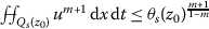
It is of interest to compare these two approaches and we restrict ourselves to the singular case \(\frac{(n-2)_{+}}{n+2}< m<1\) in the discussion. In [7] the authors introduced a certain intrinsic cylinders of the form
and used this kind of cylinders to study the boundedness, the Hölder continuity and the Harnack inequality of nonnegative weak solutions to porous medium equations. The intrinsic scaling method in [10] is very close to this kind of idea and the intrinsic cylinder takes the form

In fact, if we use a dimensional analysis, then the relation in (1.2) actually implies \([\theta]=[u]^{1-m}\), which is similar to (1.1). This enables us to use some ideas from [7] in this approach. Motivated by the proof of [7, Proposition B.4.1], Gianazza and Schwarzacher obtained a mean value result for nonnegative weak solutions [10, Proposition 5.2], which is a key ingredient in the proof of the reverse Hölder inequality in the degenerate regime. Therefore, the approach in [10] relies heavily on the regularity of the solution and this is the weak point in the study of the higher integrability. In fact, the intrinsic cylinder (1.2) shows no information for the spatial gradient. Heuristically, the intrinsic cylinder should be modified so that the factor θ should be related to the spatial gradient of \(u^{m}\). To this end, we apply the dimensional analysis again. We first note that the dimensional relation
holds. From (1.2), we obtain the dimensional relation for the time direction as follows:
Heuristically, the modified intrinsic cylinder should be taken in the following form:
However, the disadvantage of using this kind of cylinders lies in the fact that we cannot treat \(Q_{r,\theta^{1-m} r^{\frac{m+1}{m}}}(z_{0})\) locally. In fact, if \([Du^{m}]\to+\infty\), then \(|\Lambda_{\theta ^{1-m} r^{\frac{m+1}{m}}}(t_{0})|=2\theta^{1-m} r^{\frac{m+1}{m}}\to +\infty\) for any fixed \(r>0\). To this end, we set \(\varrho ^{\frac {m+1}{m}}=\theta^{1-m} r^{\frac{m+1}{m}}\) and consider the cylinders of the form
This kind of cylinders should be the correct form for the study of higher integrability of singular porous medium equations. This idea was also used in [14] to study the higher integrability of singular parabolic systems with non-standard growth. In [2] the authors considered the intrinsic cylinders of the form

which are compatible with (1.3). On the other hand, a key ingredient in the approach [1, 2] is an application of the properties of the boundary term
which was first introduced by Bögelein et al. [3]. In summary, there are some differences between these two approaches and the second approach has more advantages.
Recently, Cho and Scheven [5, 6] proved the higher integrability of weak solutions to obstacle problems related to the porous medium equation and their proofs followed the approach in [1, 2]. In [6] the authors used the boundary term (1.5) to establish an energy estimate and a gluing lemma for weak solutions of the obstacle problem. Moreover, the intrinsic cylinders in [6] takes the form (1.4). Admittedly, the approach in [2] is effective in treating the higher integrability of obstacle problem for the singular porous medium equation, but it is natural to try to use the old idea in [10] to study the same problem. To this end, the present work is intended as an attempt to follow the approach in [10] to establish a self-improving result for the obstacle problem. In this paper, we shall use the intrinsic cylinder of the type (1.2) and we will not make any use of boundary term (1.5) which is a basic tool in [1, 2, 5, 6]. The result of this paper was first announced in [15].
The present paper is built up as follows. In Sect. 2, we set up notations and state the main result. Section 3 presents some preliminaries and we explain the construction of the sub-intrinsic cylinders. In Sect. 4, we establish the energy estimates, while in Sect. 5 we prove a gluing lemma which describes the difference of two spatial averages. In Sect. 6, we establish the intrinsic reverse Hölder inequalities for the gradient on intrinsic cylinders. Finally the proof of the main result is presented in Sect. 7. Throughout this paper, we also compare our arguments with [2, 6, 10].
2 Statement of the main result
In the present section, we introduce the notations and give the statement of the main result. Throughout the paper, we assume that Ω is a bounded domain in \(\mathbb{R}^{n}\) with \(n\geq2\). For \(T>0\), let \(\Omega_{T}\) denote the space-time cylinder \(\Omega\times(0,T)\). Given a point \(z_{0}=(x_{0},t_{0})\in\mathbb{R}^{n+1}\) and two parameters \(r, s>0\), we set \(B_{r}(x_{0})=\{x\in\mathbb{R}^{n}: |x-x_{0}|< r\}\), \(\Lambda_{s}(t_{0})=(t_{0}-s,t_{0}+s)\) and \(Q_{r,s}(z_{0})=B_{r}(x_{0})\times\Lambda_{s}(t_{0})\). If the reference point \(z_{0}\) is the origin, then we simply write \(B_{r}\), \(\Lambda_{s}\) and \(Q_{r,s}\) for \(B_{r}(0)\), \(\Lambda_{s}(0)\) and \(Q_{r,s}(0)\). In this work we study obstacle problems related to the quasilinear parabolic equations of the form
Here, the vector field A is only assumed to be measurable and satisfies
where \(\nu_{0}\) and \(\nu_{1}\) are fixed positive constants. Throughout the work, we only consider the singular case \(m\in (\frac{(n-2)_{+}}{n+2},1 )\). The obstacle problem for the porous medium type equation (2.1)–(2.2) can be formulated as follows. Given an obstacle function \(\psi:\Omega_{T}\rightarrow\mathbb{R}_{+}\) with \(D\psi^{m}\in L^{2}(\Omega_{T})\) and \(\partial_{t}\psi^{m}\in L^{\frac{m+1}{m}}(\Omega_{T})\), we define the function classes
and \(K_{\psi}^{\prime}= \{v\in K_{\psi}:\partial_{t}v^{m}\in L^{\frac {m+1}{m}}(\Omega_{T}) \}\). Let \(\alpha\in W_{0}^{1,\infty}([0,T],\mathbb{R}_{+})\) be a cut-off function in time and \(\eta\in W_{0}^{1,\infty}(\Omega,\mathbb{R}_{+})\) be a cut-off function in space. We define
The definition of weak solutions to the obstacle problems related to the porous medium equation was first introduced by Bögelein et al. [3]. Cho and Scheven [4] later extended the definition to the general quasilinear structure. In this paper, we adopt the definition from [4].
Definition 2.1
([4])
A nonnegative function \(u\in K_{\psi}\) is a local weak solution to the obstacle problem related to the porous medium type equation (2.1)–(2.2) if and only if the variational inequality
holds true for any \(v\in K_{\psi}^{\prime}\), any cut-off function in time \(\alpha\in W_{0}^{1,\infty}([0,T],\mathbb{R}_{+})\) and any cut-off function in space \(\eta\in W_{0}^{1,\infty}(\Omega,\mathbb{R}_{+})\).
In this work, we shall make two regularity assumptions on the obstacle function under consideration. More precisely, we assume that the obstacle function ψ satisfies the following regularity properties:
-
(1)
The function \(\psi^{m}\) is locally Lipschitz continuous in \(\Omega_{T}\).
-
(2)
The time derivative \(\partial_{t}\psi^{1-m}\) is locally bounded in \(\Omega_{T}\).
The first assumption will be needed for the proof of Lemma 6.2 in Sect. 6, and the second assumption will be used to simplify estimating the weighted spatial averages from Sect. 5. We emphasize that the second assumption can be removed, but the proof is too long to give here. We refer the interested reader to Remark 5.4, which explains the idea of the proof.
According to [4], the assumption (1) implies that the weak solution u is locally bounded and Hölder continuous in \(\Omega_{T}\). There is no loss of generality in assuming
for all \((x,t)\in\Omega_{T}\). For simplicity of notation, we write \(\Psi=\psi^{m+1}+|\partial _{t}\psi^{m}|^{\frac{m+1}{m}}+|D\psi^{m}|^{2}\). We are now in a position to state our main theorem.
Theorem 2.2
Let \(\mathfrak {z}_{0}\in\Omega_{T}\)be a fixed point, and let \(R<1\)be a fixed positive number such that \(Q_{8R,64R^{2}}(\mathfrak {z}_{0})\subset\Omega_{T}\). Assume that there exists a constant \(M_{0}>0\)such that
Let u be a nonnegative weak solution to the obstacle problem in the sense of Definition 2.1that satisfies (2.4). Then there exists a constant \(\varepsilon =\varepsilon (n,m,\nu_{0},\nu_{1})>0\)such that

where the constant γ depends only upon n, m, \(\nu_{0}\)and \(\nu_{1}\).
Remark 2.3
Contrary to [6], our assumption (2.5) is much stronger than [6, (2.9)]. However, the Lipschitz continuity of \(\psi^{m}\) will be used to establish a mean value result for the nonnegative weak solutions and this condition seems to be optimal for the study of the obstacle problem if we follow the approach in [10].
Remark 2.4
Contrary to [10, Theorem 7.4], which established a Calderón–Zygmund type estimate for the porous medium equation, we only derive the reverse Hölder inequality for the obstacle problem. Finally, for the proof of Theorem 2.2, we will write \(\mathfrak {z}_{0}=(0,0)\) for simplicity of presentation.
3 Preliminary material
In this section, we provide some preliminary lemmas. All the materials in this section are stated without proof. We first note that the weak solution to the obstacle problem may not be differentiable in the time variable. In order to handle the problem with the time derivative, we will use the following time mollification. For a fixed \(h>0\), we set
where \(v\in L^{1}(\Omega_{T})\). Next, we recall the inequalities which were obtained from [10, Proposition 2.1].
Lemma 3.1
([10, Proposition 2.1])
Suppose that \(u, c\geq0\)and \(0< m<1\), we have
As mentioned earlier, we will not make use of the boundary term (1.5). Instead, we will use Lemma 3.1 to establish the energy estimates and a gluing lemma for the nonnegative weak solutions to the obstacle problem. Furthermore, we recall the definitions of intrinsic and sub-intrinsic cylinders which were introduced from [10, Sect. 3].
Definition 3.2
([10])
Let \(z_{0}\in\Omega_{T}\) be a fixed point, and let \(r, \theta>0\) such that \(Q_{r,\theta r^{2}}(z_{0}) \subset\Omega_{T}\). We say that \(Q_{r,\theta r^{2}}(z_{0})\) is a sub-intrinsic cylinder if and only if the following inequality holds:

where the constant \(K_{1}\geq1\). Moreover, we say that \(Q_{r,\theta r^{2}}(z_{0})\) is an intrinsic cylinder if and only if

holds for some constant \(K_{2}\geq1\).
At this point, we follow the idea in [10] to construct the sub-intrinsic cylinders which will be used in the covering argument in Sect. 7. Let \(z_{0}=(x_{0},t_{0})\in\Omega_{T}\) be a point such that \(Q_{R,R^{2}}(z_{0}) \subset\Omega_{T}\). For any \(s\in(0,R^{2}]\), we denote by \(\tilde{r}(s)\) the quantity
Let \(b_{0}=(n+2)(m+1)-2n\) and let \(\hat{b}\in(0,\min\{b_{0},\frac{1}{2}\})\). According to the proof of [10, Lemma 3.1], the function \(\tilde{r}(s)\) is continuous and this enables us to introduce the radius
for any \(s\in(0,R^{2}]\). Subsequently, we write \(Q_{s}(z_{0})=Q_{r(s),s}(z_{0})\) and denote by \(\theta_{s}(z_{0})\) the quantity
If \(z_{0}=(0,0)\), then we abbreviate \(Q_{s}:= Q_{s}((0,0))\) and \(\theta _{s}:=\theta_{s}((0,0))\). We now summarize the results obtained from [10] for this kind of cylinder as follows.
Lemma 3.3
([10])
Fix a point \(z_{0}\in\Omega _{T}\)and assume that \(Q_{R,R^{2}}(z_{0}) \subset\Omega_{T}\). Let \(s\in(0,R^{2}]\)and \(r(s)\)be the radius constructed via (3.3)–(3.4). Then the cylinder \(Q_{s}(z_{0})\)is sub-intrinsic and satisfies the following property:
-
(1)
 .
.
 .
.For \(s,\sigma\in(0,R^{2}]\)and \(s<\sigma\), we have the properties for the concentric cylinders \(Q_{s}(z_{0})\)and \(Q_{\sigma}(z_{0})\)as follows:
-
(2)
\(r(s)\leq (\frac{s}{\sigma} )^{\hat {b}}r(\sigma)\)and \(r(s)\to0\)as \(s\downarrow0\).
-
(3)
If
 holds for any \(\tau\in (s,\sigma)\), then $$\theta_{\tau}(z_{0})\leq \biggl(\frac{\tau}{\sigma} \biggr)^{\beta}\theta_{\sigma}(z_{0}), $$
where \(\beta=1-2\hat{b}>0\).
-
(4)
If \(\sigma=ks\)for some \(k\geq1\), then we have
$$ \begin{gathered}r(s)\leq k^{-\hat{b}}r(ks)\leq k^{\hat{a}-\hat{b}}r(s), \\ \theta_{ks}(z_{0})\leq k^{\beta} \theta_{s}(z_{0})\leq k^{\beta +2\hat{a}} \theta_{ks}(z_{0}), \end{gathered} $$where \(\hat{a}=\hat{b}+\frac{2}{2(m+1)-(1-m)n}\).
-
(5)
If \(\sigma=ks\)for some \(k\geq1\)and \(Q_{s}(z_{0})\)is intrinsic, then also the cylinder \(Q_{\sigma}(z_{0})\)is intrinsic.
 holds for any
 Let \(\mathfrak {z}_{0}\in\Omega_{T}\)be a point such that \(Q_{8R,64R^{2}}(\mathfrak {z}_{0})\subset\Omega_{T}\)and assume that, for some \(K\geq1\),

Then, for any \(z\in Q_{4R,16R^{2}}(\mathfrak {z}_{0})\), we have the following global estimate:
-
(6)
\(1\leq\theta_{R^{2}}(z)\leq cK^{2(m+1)\bar{a}}\), where \(\bar{a}=\frac{1}{2(m+1)+n(m-1)}\)and \(c=c(n,m)\).
Furthermore, if \(y,z\in Q_{4R,16R^{2}}(\mathfrak {z}_{0})\)and \(Q_{r(s,z),s}(z)\cap Q_{r(s,y),s}(y)\neq\emptyset\), then there exists a constant \(\hat{c}=\hat{c}(n,m,K)>1\)such that for any \(0< s\leq\frac{R^{2}}{2\hat{c}}\)we have
-
(7)
\(Q_{r(s,z),s}(z)\subset Q_{r(\hat{c}s,y),\hat{c}s}(y)\)and \(Q_{r(s,y),s}(y)\subset Q_{r(\hat{c}s,z),\hat{c}s}(z)\).
In the applications, we can use the assumption (2.4) to deduce that

This enables us to take \(K=1\) when we apply Lemma 3.3(6) and (7). As indicated in [10], the properties (4) and (7) imply the following Vitali-type covering property which will be used only in Sect. 7.
Lemma 3.4
([10])
Let \(V\subset Q_{4R,16R^{2}}(\mathfrak {z}_{0})\)and let \(Q_{r(s,z),s}(z)\)be the sub-intrinsic cylinder as in Lemma 3.3. Let \(\mathcal{F}=\{ Q_{r(s,z),s}(z): z\in V\}\)be a covering of V. Then there exist a countable family \(\mathcal{G}=\{Q_{r(s_{i},z_{i}),s_{i}}(z_{i})\} _{i=1}^{\infty}\)of disjoint cylinders in \(\mathcal{F}\)and a constant \(\chi=\chi(n,m)>1\)such that
Remark 3.5
In the construction of the sub-intrinsic cylinder \(Q_{s}(z_{0})\), we first determine the radius r in terms of a fixed \(s>0\) and this determines the value of \(\theta_{s}(z_{0})\) by (3.5). As mentioned in the introduction, this kind of sub-intrinsic cylinders shows no information for the spatial gradient. In contrast to [2, Sect. 7.1], the inequality in (3.3) is coincident with
which is the inequality in the definition of \(\tilde{\theta}_{\varrho }\) in [2, Sect. 7.1]. In [2, Sect. 7.1] the authors first determine the value of \(\theta_{z_{0};\varrho }\) in terms of a fixed \(\varrho >0\) and a quantity \(\lambda_{0}\). This determines a new type of sub-intrinsic cylinder \(Q_{\varrho }^{(\theta _{z_{0};\varrho } )}(z_{0})\) and this construction also establishes a relationship between the factor \(\theta_{\varrho }\) and the spatial gradient.
4 Caccioppoli type inequalities
The aim of this section is to establish energy estimates for the weak solution of the obstacle problem. Here, we state and prove the energy estimates on the condition that the function Ψ is locally integrable in \(\Omega_{T}\). Our main result in this section states as follows.
Lemma 4.1
Let \(0< m<1\)and let u be a nonnegative weak solution to the obstacle problem in the sense of Definition 2.1. Let \(z_{0}=(x_{0},t_{0})\in\Omega_{T}\)be a point such that \(Q_{r_{1},s_{1}}(z_{0})\subset Q_{r_{2},s_{2}}(z_{0})\subset\Omega_{T}\). Assume that \(\phi\in C_{0}^{\infty}(B_{r_{2}}(x_{0}))\)and \(0\leq\phi\leq1\). Then there exists a constant \(\gamma=\gamma(m,\nu_{0},\nu_{1})>0\)such that for any \(c\geq0\)we have
Moreover, for any \(c\geq0\)we have
where the constant γ depends only upon \(\nu_{0}\), \(\nu_{1}\)and m.
Proof
We begin with the proof of (4.1), which is the most difficult part of the proof. In the variational inequality (2.3) we choose
as a comparison map, where the function \(\psi_{c}\) is defined by \(\psi_{c}^{m}=\max\{c^{m},\psi^{m}\}\). It is easy to check that \(v\in K_{\psi}^{\prime}\). We first remark that, since \(u\geq\psi\), the two superlevel sets \(\{ u\geq c\}\) and \(\{u\geq\psi_{c}\}\) are equal. More precisely, the relation
holds true for any \(t\in\Lambda_{s_{2}}(t_{0})\). Let \(\eta=\phi^{2}\) and \(\alpha\in W_{0}^{1,\infty}([0,T],\mathbb{R}_{+})\) be a fixed cut-off function which will be determined later.
We now proceed to establish an energy estimate from the variational inequality (2.3). For the first term on the left-hand side of (2.3) we compute
In view of (4.3), we deduce \(\partial_{t}v^{m}=\partial_{t}[\![u^{m}]\!]_{h}\chi_{\{[\![u^{m}]\!]_{h}\leq\psi _{c}^{m}\}}+\partial_{t}\psi_{c}^{m}\chi_{\{[\![u^{m}]\!]_{h}>\psi_{c}^{m}\}}\) and the second term on the right-hand side of (4.5) is estimated above by
where we have used the identity \(\partial_{t}[\![u^{m}]\!]_{h}=h^{-1}(u^{m}-[\! [u^{m}]\!]_{h})\). Noting that
we have
Integrating by parts, we obtain
Combining (4.6) with (4.5), we infer that
with the obvious meaning of I, II, III, IV and V. Observe that \([\![\psi ^{m}]\!]_{h}\to\psi^{m}\) and \([\![u^{m}]\!]_{h}\to u^{m}\) uniformly in \(\Omega_{T}\) as \(h\downarrow0\), since ψ and u are locally continuous. We apply Lebesgue’s dominated convergence theorem to obtain \(I+\mathit{II}+\mathit{III}+ \mathit{IV}\to0\) as \(h\downarrow0\). It remains to treat the term V.
Noting that
we use integration by parts to get
with the obvious meaning of \(V_{1}\) and \(V_{2}\). We first observe that
since \([\![u^{m}]\!]_{h}\to u^{m}\) uniformly in \(\Omega_{T}\) as \(h\downarrow0\). Our next aim is to obtain lower and upper bounds for \(V_{1}\). To this end, we need to determine the cut-off function in time \(\alpha(t)\). For a fixed time level \(t_{1}\in\Lambda_{s_{1}}(t_{0})\subset(0,T)\), we define
where \(0<\varepsilon \ll1\). We now turn our attention to the estimate of \(V_{1}\). From (3.1), we find that
Applying Lebesgue’s dominated convergence theorem, we pass to the limit \(h\downarrow0\) on the right-hand side and conclude that
From the preceding arguments, we infer from (4.7) that, for any \(t_{1}\in\Lambda_{s_{1}}(t_{0})\), we have
with the obvious meaning of VI, VII and VIII. To estimate VI, we note that \(u-\psi_{c}\leq u-c\) on the set \(\{u\geq\psi_{c}\}\). From this inequality and (4.4), we conclude that
We now come to the estimate of VII. We first observe that \(\{\psi>c\}\subset\{u>c\}\), \(\partial_{t} \psi_{c}=\partial_{t}(\psi^{m}-c^{m})_{+}\) and \(u=(u^{m})^{\frac{1}{m}}\leq2^{\frac{1-m}{m}} ((u^{m}-c^{m})_{+}^{\frac{1}{m}}+c)\). From this inequality, we conclude that
since \((u^{m}-c^{m})_{+}^{\frac{m+1}{m}}\leq(u-c)_{+}(u^{m}-c^{m})_{+}\). Our next aim is to find a lower bound for VIII. We fix \(t_{1}\in\Lambda_{s_{1}}(t_{0})\) and consider the superlevel set \(\{B_{r_{2}}(x_{0}): u(x,t_{1})\geq\psi_{c} (x,t_{1}) \}\). On this set, \(u\geq c\) and we have
Denote \(L_{1}=(u-c)(\psi^{m}-c^{m})_{+}\) and \(L_{2}=(\psi-c)_{+}(u^{m}-c^{m})\). To estimate \(L_{1}\), we first consider the easy case \((\psi^{m}-c^{m})_{+}\leq 4^{-1}(u^{m}-c^{m})\). In this case, we get
While in the case \((\psi^{m}-c^{m})_{+}>4^{-1}(u^{m}-c^{m})\), we have \(\psi\geq c\) and \(u^{m}<4\psi^{m}-3c^{m}\leq4\psi^{m}\). Since \(\frac{1}{m}>1\), we find that
where the constant γ depends only on m. Combining this estimate with (4.13), we obtain
Next, we consider the estimate of \(L_{2}\). In the case \((\psi-c)_{+}\leq 4^{-1}(u-c)\), we have
In the case \((\psi-c)_{+}> 4^{-1}(u-c)\), we see that \(\psi\geq c\) and \(u<4\psi-3c\). Furthermore, we conclude that there exists \(\gamma =\gamma(m)\) such that
Combining this estimate with (4.15), we have shown that the estimate
holds in any case. Therefore, we conclude from (4.12), (4.14) and (4.16) that the inequality
holds for any \(x\in\{B_{r_{2}}(x_{0}): u(x,t_{1})\geq\psi_{c} (x,t_{1}) \}\). We now turn our attention to the estimate of VIII. It follows from (4.4) that
since \(\phi\leq1\). It remains to treat the second term on the right-hand side of (4.17). For \(t_{1}\in\Lambda_{s_{1}}(t_{0})\), we obtain
Furthermore, we deduce from (4.17) the estimate
From (4.9)–(4.11) and (4.18), we are led to the conclusion that there exists a constant \(\gamma=\gamma(m)\) such that
Another step in the proof of (4.1) is to find an estimate for diffusion term in (2.3). We first note that
where
By Young’s inequality and the growth assumption of the vector field A, we obtain the estimate for the first term on the right-hand side
where the constant γ depends only upon \(\nu_{0}\) and \(\nu_{1}\). Next, we consider the second term on the right-hand side of (4.20). Using Young’s inequality and the ellipticity assumption of the vector field A, we deduce
Furthermore, we need to consider the estimate of the gradient on the superlevel set \(\{u>c\}\). Since \(u\geq\psi\), we have
and therefore \(Du^{m}=D\psi^{m}\) a.e. on \(\{z\in\Omega_{T}:c< u(z)\leq\psi _{c}\}\). This implies that
Combining the estimates (4.20)–(4.23), we conclude that
This estimate together with (4.19) yield
for any \(t_{1}\in\Lambda_{s_{1}}(t_{0})\). This proves the desired estimate (4.1) by taking the supremum over \(t_{1}\in\Lambda_{s_{1}}(t_{0})\) in the first term and \(t_{1}=t_{0}+s_{1}\) in the second one.
Finally, we address the proof of (4.2). This result will be proved if we can show that the estimate
holds for any \(t_{1}\in\Lambda_{s_{1}}(t_{0})\). In order to prove this estimate, we will work on the sublevel set \(\{u< c\}\) and the argument is similar in spirit to [4, Lemma 3.1 (ii)] and [10, Lemma 4.1].
According to the proof of [4, Lemma 3.1 (ii)], we set
as a comparison map and obtain
where the cut-off function α is defined in (4.8) and \(\eta=\phi^{2}\). To estimate the third term on the right-hand side, we infer from (3.2) that
At this point, the desired estimate (4.24) follows from a standard argument (see for instance [10, page 26-28] and [4, page 12]) and we omit the details. The proof of the lemma is now complete. □
Remark 4.2
In contrast to [6, Lemma 4.1], the inequality (4.2) is indeed a special case of [6, (4.1)]. Here, we set \(f\sim g\) if \(\gamma^{-1}g\leq f\leq\gamma g\) holds for some \(\gamma=\gamma(m)>0\). From [6, (4.6)], we have
The main novelty with respect to [6, Lemma 4.1] is that we have also established an energy estimate (4.1) for the truncated function \((u-c)_{+}(u^{m}-c^{m})_{+}\) by using (4.3) as a comparison map. This inequality will be used to prove a boundedness result for the nonnegative weak solutions in Sect. 6. Our proof of (4.2) also encompasses the use of the boundary term (1.5) which is the basic tool in the proof of [6, Lemma 4.1].
5 Estimates on the spatial average
This section is devoted to the study of a gluing Lemma, which concerns weighted mean values of the weak solution on different time slices. We first state and prove the gluing lemma on the condition that the functions Ψ and \(\partial _{t} \psi^{1-m}\) are locally integrable. Let B be an open ball in \(\Omega\subset\mathbb{R}^{n}\) and let \(\eta \geq0\) be a smooth function supported in the compact set B̄. Here and subsequently, we define
The following lemma is our main result in this section.
Lemma 5.1
Let u be a nonnegative weak solution to the obstacle problem in the sense of Definition 2.1. Fix a point \(z_{0}=(x_{0},t_{0})\in\Omega_{T}\)and assume that \(Q_{r_{1},s}(z_{0})\subset Q_{r_{2},s}(z_{0}) \subset\Omega_{T}\). Let \(\xi\in C_{0}^{\infty}(B_{r_{2}}(x_{0}))\), \(0\leq\xi \leq1\)in \(B_{r_{2}}(x_{0})\), \(\xi\equiv1\)in \(B_{r_{1}}(x_{0})\)and \(|D\xi|\leq2(r_{2}-r_{1})^{-1}\). Let \(\Psi_{1}\)be the quantity

Then, for any \(t_{1}, t_{2}\in\Lambda_{s}(t_{0})\), we have

and

where the constant γ depends only upon \(\nu_{0}\), \(\nu_{1}\)and m.
Remark 5.2
Before we address the proof of Lemma 5.1, we first note that the proof of this lemma can be achieved along the lines of the proof of [6, Lemma 4.2]. However, since we are dealing with the nonnegative weak solutions, we give here a much simpler proof based on the inequality (3.2). Our proof makes no use of the boundary term (1.5) which plays a crucial role in the proof of [6, Lemma 4.2].
Proof of Lemma 5.1
Our proof is in the spirit of [5, Lemma 3.2, Lemma 4.1]. Without loss of generality, we may assume that \(t_{1}< t_{2}\). In the variational inequality (2.3) we choose \(\eta =\xi\) as a cut-off function in space and, motivated by the proof of [5, Lemma 3.2], we choose
as a cut-off function in time, where \(0<\varepsilon \ll1\). According to the argument in [5, page 19], it suffices to prove the lemma in the case \((u(t_{1}))^{\xi}_{B_{r_{2}}(x_{0})}<(u(t_{2}))^{\xi}_{B_{r_{2}}(x_{0})}\). Let μ be a fixed positive constant, which will be determined later. We follow the argument in [5, page 14-15] to deduce
where we abbreviated
and the term \(I_{h}\) tends to zero as \(h\downarrow0\). To estimate L, we use integration by parts to obtain
with the obvious meaning of \(L_{1}\) and \(L_{2}\). By Lebesgue’s dominated convergence theorem, we see that \(L_{1}\) tends to zero as \(h\downarrow 0\). Next, we consider the estimate for \(L_{2}\). To this end, we use integration by parts to obtain
with the obvious meaning of \(L_{3}\) and \(L_{4}\). From Lemma 3.1 (3.2), there exists a constant \(\gamma =\gamma(m)\) such that
since
Moreover, we note that

and this implies

Next, we consider the estimate for \(L_{4}\). From (5.3) and Hölder’s inequality, we deduce

To estimate the diffusion term, we infer from the argument in [5, page 17] that
Combining the estimates above, we apply Young’s inequality to conclude that

holds for any \(\mu>0\). At this stage, we set \(0<\delta\ll1\). In the estimate (5.5) we choose

This concludes the estimate (5.1) by passing to the limit \(\delta\downarrow0\). Finally, if we choose

then the desired estimate (5.2) follows by passing to the limit \(\delta\downarrow0\). This finishes the proof of the lemma. □
Moreover, if \(\psi^{m}\) is locally Lipschitz continuous and \(\partial _{t}\psi^{1-m}\) is locally bounded, then we can rewrite the estimates (5.1) and (5.2) in the following ready-to-use form.
Corollary 5.3
Suppose that
for some \(M_{0}>1\). Then, for any \(t_{1}, t_{2}\in\Lambda_{s}(t_{0})\), we have

and

where the constant γ depends only on \(\nu_{0}\), \(\nu_{1}\)and m.
This corollary is a direct consequence of Lemma 5.1 and the proof is omitted. For the applications, we shall use (5.8) and (5.9) to the analysis of degenerate and non-degenerate regimes in Sect. 6, respectively. The purpose of [6, Lemma 4.2] is to establish a Sobolev–Poincaré type inequality [6, Lemma 4.3] for the obstacle problem which is similar to [2, Lemma 5.1]. The quantity μ in [6] is also determined in two alternatives, which are [6, (4.35)] and [6, (4.36)]. It is easy to check that our choice of μ in (5.7) is coincident with the choice of μ in [6, page 27] but (5.6) is different from [6, page 30]. Compared with [6, Lemma 4.3], our concepts of degenerate and non-degenerate regimes have no concern with the spatial gradient.
Remark 5.4
Motivated by the proof of [6, Lemma 4.2], we can remove the assumption that \(\sup_{Q_{8R,64R^{2}}(\mathfrak {z}_{0})}|\partial_{t}\psi^{1-m}|<+\infty\). To this end, it is sufficient to improve the estimate (5.4). In the case \(m\leq\frac{1}{3}\), we have \(|\partial_{t}\psi ^{1-m}|=\frac{1-m}{m}|\psi^{1-2m}\partial_{t}\psi^{m}|\leq\frac {1-m}{m}|\partial_{t}\psi^{m}|\), since \(\psi\leq u\leq1\). From (5.4), we deduce

In the case \(m>\frac{1}{3}\), we use Hölder’s inequality and the energy estimate (4.1) to deduce

In the analysis of the non-degenerate regime, we could use (5.10) for the choice of μ as in (5.7). For the treatment of the degenerate regime, we use Young’s inequality to obtain

and the quantity μ can be determined by (5.6). The proofs are left to the reader.
6 Reverse Hölder-type inequalities
The proof of the reverse Hölder inequalities on intrinsic cylinders follows from the analysis of two complementary cases. Following [10], we give the definitions of degenerate and non-degenerate regimes.
Definition 6.1
([10])
Fix a point \(z_{0}\in\Omega_{T}\) and suppose that \(Q_{R,R^{2}}(z_{0})\subset \Omega_{T}\). Let \(\varepsilon >0\) be a fixed number and let \(Q_{s}(z_{0})\) be an intrinsic cylinder constructed in Sect. 3. We call a cylinder \(Q_{s}(z_{0})\) degenerate if and only if

holds true. Moreover, we call a cylinder \(Q_{s}(z_{0})\) non-degenerate if and only if the following inequality holds:

Next, we consider separately the degenerate and non-degenerate case. In contrast to [2, Sect. 6], our assumptions (6.1)–(6.2) show no information for the spatial gradient of the solution and the intrinsic cylinder under consideration takes the form (1.2). Our approach relies heavily on the regularity of the solution.
6.1 The degenerate alternative
This subsection deals with the degenerate case. We first establish a boundedness result analogue to [10, Proposition 5.2]. The local boundedness for weak solutions to the singular parabolic obstacle problems was first proved by Cho and Scheven [4]. Here, we present a mean value type estimate and our proof is in the spirit of [10, Proposition 5.2].
Lemma 6.2
Let u be a nonnegative weak solution to the obstacle problem in the sense of Definition 2.1. Fix a point \(z_{0}\in\Omega_{T}\)and suppose that \(Q_{R,R^{2}}(z_{0})\subset \Omega_{T}\). Let \(0< s\leq\frac{1}{2}R^{2}\)and \(r(2s)\)makes sense. Assume that the cylinder \(Q_{s}(z_{0})\)is intrinsic and
Then there exists a constant \(\gamma=\gamma(n,m,\nu_{0},\nu_{1})\)such that

Proof
There is no loss of generality in assuming \(z_{0}=(x_{0},t_{0})=(0,0)\). For \(j=0,1,2,\dots\), set \(s_{j}=s+2^{-j}s\), \(r_{j}=r(s_{j})\), \(B_{j}=B_{r_{j}}\) and \(Q_{j}=Q_{r_{j},s_{j}}\). We define a sequence of numbers \(k_{j}^{m}=k^{m}-2^{-j}k^{m}\), where \(k>0\) is to be determined. Let \(\zeta_{j}=\zeta_{j}(x)\) be a smooth function such that \(\zeta_{j}\in C_{0}^{\infty}(B_{j})\), \(0\leq\zeta_{j}\leq1\), \(\zeta_{j}\equiv1\) in \(B_{j+1}\) and \(|D\zeta_{j}|\leq2(r_{j}-r_{j+1})^{-1}\). We now apply the Caccioppoli estimate (4.1) with \((c, \phi, Q_{r_{1},s_{1}}, Q_{r_{2},s_{2}})\) replaced by \((k_{j+1}, \zeta_{j}, Q_{j+1}, Q_{j})\) to obtain
We first observe from Lemma 3.3(5) that all the cylinders \(Q_{j}\) are intrinsic. Moreover, from Lemma 3.3(4) and the assumption (6.3), we deduce
Then we follow the argument in [10, page 33-34] to impose a condition \(k\geq\theta_{2s}^{\frac{1}{1-m}}\) and obtain
Consequently, we can apply the parabolic Sobolev inequality to \((u^{m}-k_{j+1}^{m})_{+}\zeta_{j}\) on the cylinder \(B_{j}\times (-t_{j+1},t_{j+1})\), which gives
where

For more details on the proof of (6.5), we refer the reader to [10, page 34]. According to the argument in [10, page 34], we obtain \(Y_{j}\to0\) as \(j\to\infty\), provided that

where \(\gamma>1\) depends only upon n, \(\nu_{0}\), \(\nu_{1}\) and m. This proves (6.4) and the proof of Lemma 6.2 is complete. □
We remark that the intrinsic condition for \(Q_{s}(z_{0})\) is necessary in the proof of Lemma 6.2. This restricts us to work with the intrinsic cylinders in the degenerate regime. With the help of Lemma 6.2, we can now establish the reverse Hölder inequality for the degenerate regime.
Proposition 6.3
Let u be a nonnegative weak solution to the obstacle problem in the sense of Definition 2.1. Fix a point \(z_{0}\in\Omega_{T}\)and suppose that \(Q_{R,R^{2}}(z_{0})\subset \Omega_{T}\). Let \(0< s\leq\frac{1}{3}R^{2}\)and \(r(3s)\)makes sense. Assume that the cylinder \(Q_{s}(z_{0})\)is intrinsic and satisfies (6.1). Moreover, assume that \(\psi^{m}\)is locally Lipschitz continuous and
for some \(M_{0}>0\). Then there exists \(q_{1}\in(\frac{1}{2},1)\), depending only upon n and m, such that the following holds:

Proof
For abbreviation, we assume that \(z_{0}=(x_{0},t_{0})=(0,0)\). Initially, we use (4.2) from Lemma 4.1 to obtain

From Lemma 3.3(1), (2), (4) and Hölder’s inequality, we obtain

Before proceeding further, we distinguish between two cases:
Observe that the desired estimate (6.6) holds immediately in the first case. It remains to treat the second case. We first note that

Our next aim is to find an upper bound for \(s^{-1}\theta_{s}^{\frac{m+1}{1-m}}\). Let \(\eta\in C_{0}^{\infty}(B_{r(3s)})\), \(0\leq\eta\leq1\) in \(B_{r(3s)}\), \(\eta\equiv1\) in \(B_{r(2s)}\) and \(|D\eta|\leq2(r(3s)-r(2s))^{-1}\). We denote by \(\lambda_{0}\) the constant

Since \(\sup_{Q_{2s}}\Psi\leq s^{-1}\theta_{s}^{\frac{m+1}{1-m}}\), the assumptions of Lemma 6.2 are fulfilled. Applying (6.4) and Hölder’s inequality, we obtain similar to [10, Corollary 5.4] that

Next, we choose \(q_{1}\in(\frac{1}{2},1)\) such that
By Sobolev inequality and Lemma 3.3(4), we deduce

Using a similar argument to the proof of [10, Proposition 6.2], we infer from (6.1), (6.7), (6.8) and (6.10) that

where \(\alpha=\frac{2q_{1}m}{m+1}\). To estimate the second term on the right-hand side, we apply the estimate (5.8) from Corollary 5.3 to deduce

where we have used Lemma 3.3(2), (4) for the last estimate. From this, we conclude that

since \(s=\theta_{s}r(s)^{2}\). We insert this inequality in (6.11) and this implies that

with the obvious meaning of \(L_{1}\), \(L_{2}\) and \(L_{3}\). We first consider the estimate for \(L_{2}\). Since \(u\geq\psi\), we apply Lemma 3.3(1), (4) and Hölder’s inequality to deduce

This implies that
Next, we rewrite \(L_{3}\) as follows:
Combining the estimates above, we arrive at

Observe that we can reabsorb the second term \(\frac{1}{2}\frac{\theta_{s}^{\frac{m+1}{1-m}}}{s}\) on the right-hand side into the left. It follows that

At this point, we claim that

In the case \(s^{-1}\theta_{s}^{\frac{m+1}{1-m}}\leq1\), it is easy to see that (6.13) holds trivially. In the case \(s^{-1}\theta_{s}^{\frac{m+1}{1-m}}> 1\), the desired estimate (6.13) directly follows from (6.12). This proves (6.13) and the proof of Proposition 6.3 is complete. □
6.2 The non-degenerate alternative
In this subsection, we prove the reverse Hölder inequality analogue to (6.6) for the non-degenerate regime. The treatment for non-degenerate case is different from the degenerate case.
Proposition 6.4
Let u be a nonnegative weak solution to the obstacle problem in the sense of Definition 2.1. Fix a point \(z_{0}\in\Omega_{T}\)and suppose that \(Q_{R,R^{2}}(z_{0})\subset \Omega_{T}\). Let \(0< s\leq R^{2}\)and suppose that the cylinder \(Q_{s}(z_{0})\)is intrinsic and satisfies (6.2). Moreover, assume that \(\psi^{m}\)is locally Lipschitz continuous and
for some \(M_{0}>0\). Then there exists \(q_{1}\in(\frac{1}{2},1)\), depending only upon n and m, such that the following holds:

Proof
For simplicity of presentation, we assume that \(z_{0}=(0,0)\). Let us first construct a smooth function \(\eta\in C_{0}^{\infty}(B_{r(s)})\) satisfying \(0\leq\eta\leq1\) in \(B_{r(s)}\), \(\eta\equiv1\) in \(B_{r(s/2)}\) and \(|D\eta|\leq2(r(s)-r(s/2))^{-1}\). Define

where \(t\in\Lambda_{s}\). Let \(\sigma_{1}\), \(\sigma_{2}\in[\frac{1}{2},1]\) and \(\sigma_{1}<\sigma_{2}\). Applying a similar argument to the proof of [10, Proposition 6.3], we infer from (6.2) that
Furthermore, we apply the Caccioppoli estimate (4.2) with \((c, Q_{r_{1},s_{1}}, Q_{r_{2},s_{2}})\) replaced by \((\lambda, Q_{\sigma_{1}s}, Q_{\sigma_{2}s})\) to obtain

since \(r(\sigma_{2}s)-r(\sigma_{1}s)\geq c(\sigma_{2}-\sigma_{1})^{\hat{b}}r(s/2)\geq c(\sigma_{2}-\sigma_{1})r(s)\). For any \(\sigma\in[\frac{1}{2},1]\), we set

We now choose \(q_{1}\in(\frac{1}{2},1)\) satisfying (6.9). According to the proof of [10, Proposition 6.3], we infer from (6.16) that

where \(\alpha=\frac{2q_{1}m}{m+1}\). It remains to treat the third term on the right-hand side of (6.17). We first consider the case \(r(s)^{\frac{1}{m}}> \frac{s}{r(s)}\). Since \(\lambda\leq c_{2}\theta_{s}^{\frac{1}{1-m}}\), we deduce
and therefore \(r>c_{2}^{-m}\lambda^{m}\). Recalling that \(\lambda (t)=(u(t))_{B_{r(s)}}^{\eta}\), we obtain \(\lambda(t)^{m+1}\leq c(u(t)^{m+1})_{B_{r(s)}}\). Consequently, we deduce that

Next, we turn our attention to the case \(r(s)^{\frac{1}{m}}\leq\frac {s}{r(s)}\). We apply the inequality (5.9) from Corollary 5.3 to obtain

with the obvious meaning of \(L_{1}\), \(L_{2}\) and \(L_{3}\). We first consider the estimate for \(L_{1}\). From (6.15), we get

To estimate \(L_{2}\), we recall that \(u\geq\psi\). From (6.15) and Hölder’s inequality, we obtain

Finally, we address the estimate of \(L_{3}\). Recalling that \(r(s)^{\frac {1}{m}}\leq\frac{s}{r(s)}\), we have
since \(\lambda\geq c_{1}\theta_{s}^{\frac{1}{1-m}}\). Consequently, we arrive at

for any \(\sigma_{1}, \sigma_{2}\in[\frac{1}{2},1]\) and \(\sigma _{1}<\sigma_{2}\). Now, we apply the iteration result from [1, Lemma 2.1] to reabsorb the first term on the right-hand side into the left. We have thus proved the proposition. □
7 Proof of the main result
This section is devoted to the proof of Theorem 2.2. Our proof uses a certain stopping time argument which was introduced by Gianazza and Schwarzacher [10]. However, in the context of the obstacle problem, the argument is considerably more delicate. We first point out that the scaling argument does not seem to work for the obstacle problem. On the other hand, in order to use the reverse Hölder inequalities in Sect. 6, we introduce a certain localized-centered maximal function. We adopt this kind of maximal function to construct the superlevel sets of the gradient.
We now turn to the proof of Theorem 2.2. Recalling that we have assumed \(\mathfrak {z}_{0}=(0,0)\). In this case, the assumption (2.5) reads
For simplicity of presentation, we abbreviate \(Q_{2R,4R^{2}}\) to Q̂. For \(L\gg1\) to be fixed later, we introduce a localized average function

where f is a locally integrable function in \(\Omega_{T}\). Moreover, for any \(f\in L^{1}_{\mathrm{loc}}(\Omega_{T})\), we define the localized-centered maximal function as follows:
Next, we remark that this kind of one-parameter maximal function is different from the Hardy–Littlewood maximal function and it is of interest to know whether \(f(z)\leq T^{*}(f)(z)\) for almost every \(z\in\hat{Q}\). This motivates us to establish the following lemma.
Lemma 7.1
For any \(f\geq0\)with \(f\in L_{\mathrm {loc}}^{1}(\Omega_{T})\), we have
for almost every \(z\in\hat{Q}\).
Proof
Our first goal is to establish the following weak type estimate:
where the constant \(c^{\prime}\) depends only on n and m. In order to prove (7.2), we note that for any \(z\in\hat{Q}\cap \{T^{*}(f)(z)>\lambda \}\) there exists \(s_{z}\in(0,L^{-1}R^{2}]\) such that

Moreover, the collection \(\{Q_{s_{z}}(z): z\in\hat{Q}\cap \{ T^{*}(f)(z)>\lambda \}\}\) forms a covering of the set \(\hat{Q}\cap \{T^{*}(f)(z)>\lambda \}\). From Lemma 3.4, we find a countable subfamily \(\{Q_{s_{z_{i}}}(z_{i})\} _{i=1}^{\infty}\) of pairwise disjoint cylinders, such that
where \(\chi=\chi(n,m)\) is the constant defined in Lemma 3.4. By Lemma 3.3(4), there exists a constant \(c^{\prime}=c^{\prime}(n,m)>1\) such that
which gives (7.2). Next, we define a sequence of localized average functions

where \(s_{j}=2^{-j}L^{-1}R^{2}\). Another step in the proof is to show that the sequence \(T_{j}(f)\) converges in measure on Q̂ to f. To this end, we fix \(\varepsilon _{0}>0\). For any \(\varepsilon >0\), we choose \(g\in C_{0}(\hat{Q})\) such that \(\|g -f\chi_{\hat{Q}}\|_{L^{1}(\Omega _{T})}<\frac{1}{3c^{\prime}} \varepsilon \varepsilon _{0}\). Furthermore, there exists an integer \(N_{0}=N_{0}(\varepsilon _{0},\varepsilon ,R)\) such that for any \(j\geq N_{0}\) we have
From Lemma 3.3(2), we see that \(Q_{s_{j}}(z)\subset Q_{s_{j}^{\hat{b}}R^{1-2\hat{b}},s_{j}}(z)\) and consequently
holds for all \(j\geq N_{0}\). It follows from (7.2) that for any \(j\geq N_{0}\)
This proves that \(T_{j}(f)\) converges in measure to f. Then there exists a subsequence \(T_{j_{k}}(f)\) converging to f almost everywhere. It follows that, for almost every \(z\in\hat{Q}\),
which completes the proof. □
Furthermore, for \(\sigma_{1}, \sigma_{2}\in[1,2]\) and \(\sigma _{1}<\sigma_{2}\), we define two concentric cylinders \(\hat{Q}_{\sigma _{1}}=Q_{\sigma_{1}R,\sigma_{1}^{2}R^{2}}\) and \(\hat{Q}_{\sigma_{2}}=Q_{\sigma_{2}R,\sigma_{2}^{2}R^{2}}\). We are interested in getting estimates on such concentric cylinders. To this end, we first need the following lemma.
Lemma 7.2
Let \(z\in\hat{Q}_{\sigma_{1}}\)and \(L_{1}\geq1\). If \(L_{1}s\leq R^{2}\)and \(Q_{L_{1}s}(z)\cap(\hat{Q}_{\sigma_{2}})^{c}\neq\emptyset\), then

where

and the constant γ depends only on n, m, \(\nu_{0}\), \(\nu_{1}\)and \(L_{1}\).
The proof of Lemma 7.2 is quite similar to [10, Lemma 7.1] and so is omitted. The crucial result in our proof of Theorem 2.2 will be the following proposition, which is analogue to [10, Proposition 7.2].
Proposition 7.3
Fix a point \(z\in\hat{Q}_{\sigma_{1}}\cap \{T^{*}(|Du^{m}|^{2})(z)>\lambda \}\). Suppose that \(\lambda\geq\lambda_{0}\), where

and \(L_{1}=7\chi\). Then there exist \(q_{1}\in(\frac{1}{2},1)\), \(L=L(n,m,\nu_{0},\nu _{1})>10\chi\)and \(s_{z}\in(0,2L^{-1}R^{2}]\)such that the following holds:
-
(1)
There exists a constant \(c_{1}=c_{1}(n,m,\nu_{0},\nu_{1})\)such that
 (7.3)
(7.3) -
(2)
We have \(3\chi s_{z}\leq R^{2}\), \(Q_{3\chi s_{z}}(z)\subset\hat{Q}_{\sigma_{2}}\)and
 (7.4)
(7.4)where the constant \(c_{2}\)depends only on n, m, \(\nu_{0}\)and \(\nu_{1}\).


Proof
The proof is adapted from [10, Proposition 7.2]. For any fixed point \(z\in\hat{Q}_{\sigma_{1}}\cap \{ T^{*}(|Du^{m}|^{2})(z)>\lambda \}\), we set

It follows that

Therefore, by \(\lambda\geq\lambda_{0}>3\mu_{\sigma_{1},\sigma_{2},L_{1}}\) and Lemma 7.2, we have \(Q_{L_{1}s_{z}^{\prime}}(z)\subset\hat{Q}_{\sigma_{2}}\). Let \(L_{2}> 4\) be a constant which will be chosen later, and assume that \(L\geq5L_{2}+10\chi\). This implies that \((2s_{z}^{\prime}, L_{2}s_{z}^{\prime})\subset(0,R^{2}]\).
In order to prove (7.3), we first consider the case that there exists \(s\in(2s_{z}^{\prime}, L_{2}s_{z}^{\prime})\) such that

By Lemma 3.3(5), we infer that \(Q_{2s_{z}^{\prime}}(z)\) is intrinsic. If the cylinder \(Q_{2s_{z}^{\prime}}(z)\) is degenerate, then we choose \(s_{z}=2s_{z}^{\prime}\) and (7.3) follows from Proposition 6.3. On the other hand, if the cylinder \(Q_{2s_{z}^{\prime}}(z)\) is non-degenerate, then we choose \(s_{z}=s_{z}^{\prime}\) and (7.3) follows from Proposition 6.4. Next, we turn our attention to the case that the strict inequality

holds for any \(s\in(2s_{z}^{\prime}, L_{2}s_{z}^{\prime})\). In this case, we set \(s_{z}=s_{z}^{\prime}\) and define

By hypothesis, we see that \(\sigma_{z}\in[L_{2}s_{z}, R^{2}]\) and let \(Q_{\sigma_{z}}(z)\) be a sub-intrinsic cylinder constructed in Sect. 3. Since \(s_{z}\leq L_{2}^{-1}\sigma_{z}\), we use Lemma 3.3(3) to obtain the decay estimate
where \(\beta=1-2\hat{b}\) and \(\frac{m+1}{1-m}\beta-1>0\). Next, we invoke Lemma 4.1, takes the form

In the case \(\sigma_{z}\in[\frac{1}{12 L}R^{2}, R^{2}]\), we apply Lemma 3.3(4), (6) to obtain
Combining this with (7.5) and (7.6) we find that

which proves the estimate (7.3). Furthermore, we consider the case \(\sigma_{z}\in(L_{2}s_{z},\frac{1}{12 L}R^{2})\). In this case, the cylinder \(Q_{\sigma_{z}}(z)\) is intrinsic and satisfies

It follows that

From [10, Lemma 2.4], we find that the cylinder \(Q_{\sigma _{z}}(z)\) is degenerate. This enables us to use (6.13) from the proof of Proposition 6.1. Then there exists a constant \(\hat{\gamma}=\hat{\gamma}(n,m,\nu_{0},\nu_{1})\) such that

since \(s_{z}^{\prime}<3\sigma_{z}<L^{-1}R^{2}\). Combining this with (7.5) and (7.6) we finally arrive at

In (7.7) we choose \(L_{2}=2(2\gamma\hat{\gamma})^{\frac{1}{\frac{m+1}{1-m}\beta-1}}\) and this determines the constant
Therefore, we can reabsorb the first term on the right-hand side of (7.7) into the left and this proves the estimate (7.3).
On the other hand, for such a choice of L, we see immediately that
Finally, we address the proof of (7.4). To this end, we have to distinguish two cases, whether \(3\chi s_{z}< L^{-1}R^{2}\), or \(3\chi s_{z}\geq L^{-1}R^{2}\). In the case \(3\chi s_{z}< L^{-1}R^{2}\), the inequality (7.4) follows directly from the definition of \(s_{z}^{\prime}\). Next, we consider the second case. From Lemma 3.3(4), (6), we obtain
This implies that
and consequently

which gives (7.4). This finishes the proof of the proposition. □
With the help of Lemma 7.1 and Proposition 7.3, we are now in a position to prove the main result. The proof follows in a similar manner as the proof of [10, Theorem 7.3] and we just sketch the proof.
Proof of Theorem 2.2
Let \(\lambda\geq\lambda_{0}^{\prime}\), where

and \(c_{1}\) be the constant in (7.3) from Proposition 7.3.
For any fixed \(z\in\hat{Q}_{\sigma_{1}}\cap \{ T^{*}(|Du^{m}|^{2})(z)>\lambda \}\), let \(s_{z}\) be the positive number constructed in Proposition 7.3. We note that the collection
forms a covering of the superlevel set \(\hat{Q}_{\sigma_{1}}\cap \{ T^{*}(|Du^{m}|^{2})(z)>\lambda \}\). From Lemma 3.4, there exists a countable subfamily \(\{Q_{3s_{z_{i}}}(z_{i})\}_{i=1}^{\infty}\subset\mathcal{F}\) of pairwise disjoint sub-intrinsic cylinders, such that \(\{Q_{3\chi s_{z_{i}}}(z_{i})\}_{i=1}^{\infty}\) covers the superlevel set \(\hat{Q}_{\sigma_{1}}\cap \{T^{*}(|Du^{m}|^{2})(z)>\lambda \}\). We abbreviate \(Q_{i}=Q_{s_{z_{i}}}(z_{i})\), \(Q_{i}^{*}=Q_{3s_{z_{i}}}(z_{i})\) and \(Q_{i}^{**}=Q_{3\chi s_{z_{i}}}(z_{i})\). Next, we choose \(\eta=(16c_{1})^{-1}\). Then, for each \(i=1,2,\dots\), we infer from Proposition 7.3(1) that
and hence
Recalling that \(\{Q_{i}^{**}\}_{i=1}^{\infty}\) is a covering of the set \(\hat{Q}_{\sigma_{1}}\cap \{T^{*}(|Du^{m}|^{2})(z)>\lambda \}\), we infer from Proposition 7.3(2), Lemma 3.3(4) and (7.8) that
where the constant γ̄ depends only upon n, m, \(\nu_{0}\) and \(\nu_{1}\). Moreover, for some \(\varepsilon \in(0,1)\) to be specified later and \(k>\lambda_{0}^{\prime}\), we multiply both sides of (7.9) by \(\lambda ^{-1+\varepsilon }\) and integrate over the interval \((\lambda_{0}^{\prime},k)\) with respect to λ.
To estimate a lower bound for the left-hand side of (7.9), we use the inequality (7.1) from Lemma 7.1 to infer that \(\hat{Q}_{\sigma_{1}}\cap \{|Du^{m}|^{2}(z)>\lambda \}\subset\hat{Q}_{\sigma_{1}}\cap \{T^{*}(|Du^{m}|^{2})(z)>\lambda \}\) and consequently
Next, we address the estimate of the right-hand side of (7.9). We apply Fubini’s theorem to obtain
At this stage, we choose \(\varepsilon =\frac{1-q_{1}}{2\bar{\gamma}c_{1}^{q_{1}}\eta^{q_{1}-2}}\). Combining (7.9)–(7.11), we obtain the following estimate:

Finally, we use the iteration result from [1, Lemma 2.1] to reabsorb the first term on the right-hand side into the left, and the desired estimate (2.6) is proved by letting \(k\to \infty\). This finishes the proof of Theorem 2.2. □
Remark 7.4
The method of the proof of higher integrability in [2, Sect. 7] has its origin in [12]. However, unlike the case of parabolic p-Laplace equation, the sub-intrinsic cylinders constructed for the porous medium equation are not associated with any fixed parabolic metric. Therefore, we cannot simply use the classical results from [11] to treat this kind of cylinders. In [2, Sect. 7.3] the authors illustrate that

holds for \(\mathcal{L}^{n+1}\)-a.e. point \(z\in\mathbb{R}^{n+1}\). But the proof of this claim relies on the techniques from geometric measure theory (cf. [8, 2.9.1]). In the present section we only established the inequality (7.1) which is weaker than Lebesgue’s differentiation theorem and our approach encompasses the proof of the existence of Lebesgue points.
References
Bögelein, V., Duzaar, F., Korte, R., Scheven, C.: The higher integrability of weak solutions of porous medium systems. Adv. Nonlinear Anal. 8, 1004–1034 (2019)
Bögelein, V., Duzaar, F., Scheven, C.: Higher integrability for the singular porous medium system. J. Reine Angew. Math. (2019). https://doi.org/10.1515/crelle-2019-0038
Bögelein, V., Lukkari, T., Scheven, C.: The obstacle problem for the porous medium equation. Math. Ann. 363, 455–499 (2015)
Cho, Y., Scheven, C.: Hölder regularity for singular parabolic obstacle problems of porous medium type. Int. Math. Res. Not. (2018). https://doi.org/10.1093/imrn/rny073
Cho, Y., Scheven, C.: The self-improving property of higher integrability in the obstacle problem for the porous medium equation. Nonlinear Differ. Equ. Appl. 26, Article ID 37 (2019)
Cho, Y., Scheven, C.: Higher integrability in the obstacle problem for the fast diffusion equation. J. Math. Anal. Appl. 491(2), 1–44 (2020)
DiBenedetto, E., Gianazza, U., Vespri, V.: Harnack’s Inequality for Degenerate and Singular Parabolic Equations. Springer Monographs in Mathematics. Springer, New York (2012)
Federer, H.: Geometric Measure Theory. Die Grundlehren der mathematischen Wissenschaften, vol. 153. Springer, New York (1969)
Gianazza, U., Schwarzacher, S.: Self-improving property of degenerate parabolic equations of porous medium-type. Am. J. Math. 141(2), 399–446 (2019)
Gianazza, U., Schwarzacher, S.: Self-improving property of the fast diffusion equation. J. Funct. Anal. 277(12), 1–57 (2019)
Heinonen, J.: Lectures on Analysis on Metric Spaces. Springer, New York (2001)
Kinnunen, J., Lewis, J.L.: Higher integrability for parabolic systems of p-Laplacian type. Duke Math. J. 102, 253–271 (2000)
Kinnunen, J., Lewis, J.L.: Very weak solutions of parabolic systems of p-Laplacian type. Ark. Mat. 40, 105–132 (2002)
Li, Q.: Very weak solutions of subquadratic parabolic systems with non-standard \(p(x,t)\)-growth. Nonlinear Anal. 156, 17–41 (2017)
Li, Q.: Higher integrability for obstacle problem related to the singular porous medium equation. arXiv:2004.06177
Acknowledgements
We are grateful to the editor and referee for useful comments and suggestions.
Availability of data and materials
Not applicable.
Funding
Not applicable.
Author information
Authors and Affiliations
Contributions
The author read and approved the final manuscript.
Corresponding author
Ethics declarations
Competing interests
The authors declare that they have no competing interests.
Rights and permissions
Open Access This article is licensed under a Creative Commons Attribution 4.0 International License, which permits use, sharing, adaptation, distribution and reproduction in any medium or format, as long as you give appropriate credit to the original author(s) and the source, provide a link to the Creative Commons licence, and indicate if changes were made. The images or other third party material in this article are included in the article’s Creative Commons licence, unless indicated otherwise in a credit line to the material. If material is not included in the article’s Creative Commons licence and your intended use is not permitted by statutory regulation or exceeds the permitted use, you will need to obtain permission directly from the copyright holder. To view a copy of this licence, visit http://creativecommons.org/licenses/by/4.0/.
About this article

Cite this article
Li, Q. Higher integrability for obstacle problem related to the singular porous medium equation. Bound Value Probl 2020, 147 (2020). https://doi.org/10.1186/s13661-020-01445-x
Received:
Accepted:
Published:
DOI: https://doi.org/10.1186/s13661-020-01445-x